Keywords:Stock returns; Oil sensitivity; Risk and returns
1. Introduction
The empirical research in International Finance has focused on the sensitivity of the stockmarkets of the major oil-consuming countries to changes in the oil price. The sensitivities to
2 S. Hammoudeh, H. Li / Journal of Economics and Business 57 (2005) 1–21
oil price growth1 of stock index returns of the world’s major oil-sensitive industries and theoil-exporting countries are not well researched in this financial literature. In particular, thejury is still out on the extent of oil price sensitivity of the stock markets of the oil-exportingcountries whose governments own the oil industry, which thus has no stocks traded on stockexchanges. If sensitivity to the oil price changes is found to be significant for the individualcountry/industry and for all of them as a group, then it will be interesting to compare thissensitivity to the inherent systematic risk defined with respect to the world capital market.In this case, we seek answers to the following questions: (1) how sensitive to oil pricegrowth are the returns of the composite stock indices of the oil-exporting countries, whichhave zero oil industry equity capitalization? (2) how does the oil sensitivity of those returnscompare with that of the returns of oil-related and oil-sensitive industries such as the oil andthe transportation industries whose stocks are traded on the world’s major stock markets?(3) does oil price growth matter more than the world capital market return in influencingthe oil-sensitive stock returns? Or does oil sensitivity matter more than systematic risk?
Hammoudeh and Eleisa (2004)investigated the oil sensitivity of the stock markets (with-out including the systematic risk) for five members of the oil-rich Gulf Cooperation Council(GCC). These members are Bahrain, Kuwait, Oman, Saudi Arabia and UAE which, all ex-cept Bahrain, are major oil exporters and have oil-anchored economies. They found that ona daily basis only the Saudi stock market has a bi-directional causal or mutual predictiverelationship with oil price growth. They, on the other hand, found that the stock returnsof the smaller oil exporters, Kuwait and Oman, have no causal relationships with oil pricechanges. These results are puzzling because the GCC countries are strongly oil exports-anchored and are similar in their economic structures. Do the results have something to dowith the fact that the GCC economies are very small and their stock markets are relativelyunknown?
The above study has motivated us to extend this type of research to examine other oil-exporting countries that have larger economies and more well-established stock marketsthan the GCC countries. We also included two major oil-sensitive industries. We hope tofind more meaningful directional relations or sensitivity between the oil price growth andthe oil-sensitive stock returns. In this extension we are limited by several factors includingdaily historical data availability, relatively well-established equity markets or industries andlarger, more diversified economies. The possible country candidates that fit these criteriainclude Indonesia, Mexico, Norway, Russia and Venezuela.2 The two major oil-sensitiveindustries include the US oil industry and the transportation industry. The daily sample pe-riod considered in this paper is the period 1986–2003. This sample factor excludes Russia’smarket because its daily data starts from 1995 only.3 Venezuela cannot also be includedbecause we could not find consistent daily data that fits our lengthy sample, and Indone-sia will also be excluded because its stock index is stationary in (log of) level. We hopethat examining the oil/stock link for the oil exporters, Mexico and Norway, and the oil-sensitive oil and transportation industries would balance the results found byHammoudeh
1 Oil price growth means positive or negative percentage changes in the oil price.2 These countries’ daily oil production in million barrels and their shares of world’s oil production in 2001 are:
Indonesia 1.41 and 1.9%; Mexico 3.56 and 4.8%; Norway 3.41 and 4.6%; Russia 7.5 and 10%.3 For detailed information on the Russian stock market, seeHammoudeh, Ewing, and Zhao (2003).
S. Hammoudeh, H. Li / Journal of Economics and Business 57 (2005) 1–21 3
and Eleisa (2004), and would also further our understanding of the behavior of other oil ex-porters’ stock returns such as those of Indonesia, Russia and Venezuela. These results mayalso have general information on whether the oil-sensitive stock markets have a forecastingpower of daily oil prices, and on whether the systemic risk matters more than the oil pricesensitivity.
At the industry level, we examine the oil sensitivity of two US industry stock indices:one for the oil industry and the other for the transportation industry. These two indices are,respectively, represented by the Amex Oil Index and the NYSE Transportation Index. Theoil industry stock index includes companies engaged in oil exploration, drilling, productionand refining. The transportation industry includes airlines, trucking and railroad companies.In examining the oil price–stock linkages for those two industries, our main objective isto determine whether or not these industries have stronger links with oil prices than dothe national composite stock indices of the oil-exporting countries. The national indicesconsidered in this paper have virtually zero-oil equity market capitalization because the oilindustry is owned by governments.4 Moreover, we are interested in ascertaining whether theoil industry, which depends heavily on crude oil as its major input, has a stronger predictivepower or causal relationship with the daily oil prices than the transportation industry, whichhas stronger links with the over-all economy or vice versa.
The other primary objective of this paper is to compare, through the use of an internationalAPT model, the oil price growth sensitivity with the systematic risk relative to the worldmarket return when this market is aggregated and when it is in up and down modes. Basedon the two broad objectives, we can formulate two basic hypotheses that set the stage forour analysis.
Hypothesis 1. In a system of oil-based stock returns, there are causal or predictive re-lationships running from the oil price changes to the oil-sensitive stock returns on a dailybasis.
This hypothesis will be examined using a vector error–correction model. If in this hy-pothesis we find (which is the case) that for most of the stock returns there are directionalrelationships running from the oil price to the stock returns, then the oil price is an importantfactor in determining the oil-sensitive stock returns as a group. We will then formulate afactor model that compares the returns’ oil sensitivity with their systematic risk in bothspecifications of the world capital market. In this case we will test a second hypothesis.
Hypothesis 2. The oil-based stock markets are on a daily basis more sensitive to changesin the world oil price than to the changes in the world capital market index price regardlesswhether the world market is in an up or down mode.
This hypothesis will be tested through the use of international APT models.As a result, this paper will help to fill the gaps in the VAR and APT literatures on the
sensitivities of the oil-based stock markets. Since the period under consideration is marred
4 This case is in contrast to the Russian market for which the energy sector stock index accounts for 67% ofthe total market capitalization in 2003.
4 S. Hammoudeh, H. Li / Journal of Economics and Business 57 (2005) 1–21
by international events, this study will also examine the impact of three well-known politicaland economic events on those returns.
The main findings of this study can be summarized as follows. (1) Oil price growthleads the stock returns of all the individual oil-exporting countries and the US oil-sensitiveindustries. Moreover, the world capital index MSCI was found to simultaneously have aparticularly strong predictive power of these stock returns, pinpointing the importance ofthe systematic risk with respect to the world capital market. These results which showlong-run relationships among the variables pave the ground for using the factor model. Thismodel compares the sensitivity of the national and industry stock returns to the oil pricechanges with their sensitivities to the own market risk for the specifications of the standardaggregate world market and its up and down markets as stated inHypothesis 2. (2) Based onthe extent of returns’ positive dynamic sensitivity to oil price growth, investors interestedin the oil-sensitive stocks should invest first in the stocks of the US oil industry and thenin the Mexican stocks before they invest in the Norwegian market to take advantage ofhigher oil prices. (3) Based on the dynamic sensitivity to the world capital market, investorsshould also invest first in the US oil industry followed by the US transportation industry,Norway and then Mexico. (4) Similar to Saudi Arabia inHammoudeh and Eleisa (2004),only Norway and the world capital market index have a lead relationship with the oil price,with Norway having a positive 1 day lead and MSCI showing a negative 1 day lead. (5) Allthe stock returns display sensitivity to major economic and political events, with Norwayshowing the strongest relative sensitivity. (6) Aggressive investors and aggressive growthportfolio managers interested in oil-sensitive stocks with higher returns may be inclinedto buy stocks that belong to industries or countries with higher betas (systematic risks).Among the returns considered, the US transportation and oil industry have the highestbetas. However, those investors should be willing to accept abnormal losses in the downmarket if they invest in those oil-sensitive markets.
The organization of this paper is as follows. After this introduction, Section2 presentsa brief review of the literature that used the VEC and International APT models to studythe oil-sensitive stock markets. Section3 describes the oil and financial series used incarrying out this study and also presents their descriptive statistics. Section4 discussesthe methodology and empirical results for the unit root tests, the cointegration tests andthe error–correction models. Section5 compares the stock returns’ oil sensitivity to thesystematic risk by the means of using a factor model. Section6 concludes the paper andoffers recommendations.
2. Review of related literature
There has been a large volume of work investigating the links among internationalfinancial markets. In contrast, little work has been done on the relationships between oilprice growth and oil-sensitive stock returns, and virtually all of this work has concentrated onfew industrial countries, namely, Canada, Japan, the UK and the US. This scarcity of workcould be due to separation of knowledge and expertise in oil markets and stock markets, andalso to the difficulty of obtaining adequate high frequency data on oil-exporting countries.Most of the work has examined this relationship within the framework of a macroeconomic
S. Hammoudeh, H. Li / Journal of Economics and Business 57 (2005) 1–21 5
model, using low frequency (monthly or quarterly) data and employing a proxy for oil futuresprices.Jones and Kaul (1996)investigated the reaction of the US, Canadian, Japanese andUK stock prices to oil price shocks using quarterly data. Utilizing a standard cash-flowdividend valuation model, they found that for the US and Canada this reaction can beaccounted for entirely by the impact of the oil shocks on real cash flows. The results forJapan and the UK were not as strong.Huang, Masulis, and Stoll (1996)used an unrestrictedVAR model to examine the relationship between daily oil futures returns and daily US stockreturns. They found that oil futures returns lead some individual oil company stock returnsbut they do not have much impact on the broad-based market indices such as the S&P 500.In a more recent study,Sadorsky (1999)using monthly data (January 1947–April 1996)examined the links between the US fuel oil prices and the S&P 500 in an unrestricted VARmodel that also included the short-term interest rate and industrial production. In contrastwith the findings ofHuang et al. (1996), Sadorsky found that oil price movements areimportant in explaining movements in broad-based stock returns.
Oil price growth sensitivity and its relation to the systematic risk in the standard aggregatemodel and in the up and down markets as stated inHypothesis 2did not receive enoughattention in the empirical finance literature. This literature uses the international APT modelsto examine the impacts of global (mostly non-oil) economic and political factors on stockreturns. Examples include:Ferson and Harvey (1994), Bekaert and Harvey (1995), Heston,Rouwenhorst, and Wessels (1995), Tang and Shum (2003), andKarolyi and Stultz (2003).
3. Data description
The data used in this study include daily time series for the NYMEX 3-month oil futuresprice,5 the Morgan Stanley Capital International Index and four oil-sensitive internationalstock markets indices (US Amex Oil Index, US NYSE Transportation Index, Mexico’sIPC Index and Norway’s Oslo All-Shares Index) covering the period 2 January 1986–30September 2003. It also includes four trading day dummies and three event dummies. Wecannot use macroeconomic data for GDP and inflation because they are not available daily.
The oil futures price is a price quoted for delivering a specified quantity of any of the WestTexas Intermediate (WTI) crude oil at a specific time and place in the future.6 It is quotedin dollars and cents and its series was obtained from NYMEX. The data for internationalstock indices except MSCI were acquired from Global Financial Data. The MSCI worldindex data came from Morgan Stanley Capital International.
The 3-month futures price (NYCOF3) is traded on the NYMEX and has its underlyingphysical asset be WTI, deliverable at the end of the domestic pipeline at the Cushing,Oklahoma center. The 3-month oil futures contacts are the largest oil contacts traded in theworld.
5 We use 3-month futures oil price rather than spot price because stock markets are forward-looking. InHammoudeh and Li (2004), it was found that the dynamic causal effect runs from the 3-month futures oil price tothe spot price although the two are cointegrated. Trial runs also confirmed this.
6 The WTI spot price is the price quoted for immediate delivery of the West Texas Intermediate (WTI-Cushing)in Cushing, Oklahoma trading center. WTI is a light crude stream produced in Texas and southern Oklahoma. Itserves as a reference or a marker for pricing a number of other crude streams.
6 S. Hammoudeh, H. Li / Journal of Economics and Business 57 (2005) 1–21
The Amex Oil Stock Index (AMEXO) is designed to represent a cross-section of widelyheld stocks of corporations involved in various phases of the oil industry. The index is equallyweighted, measuring the performance of the US oil industry shares through changes in thesum of prices of 16 component stocks.
The NYSE Transportation Index (NYTRAN) includes shares of airlines, trucking andrailroads companies traded at the New York Stock Exchange. This index began on 31December 1965 and it is capitalization-weighted.
The Mexico IPC Index (MEX) includes 36 major equity securities listed and traded onthe Bolsa Mexicana. These securities are shares of companies engaged mainly in telecom-munication, construction and supermarkets and do not include oil company stocks becausethe oil industry is owned by the government. Thus, there is no oil capitalization in theIPC. The inclusion of equities in this index is based on trading value, volume and capitali-zation.
The Norway Oslo All-Shares Return Index (NOR) is a total return index. The companiesincluded in this index are weighted in relation to the market value of the portion of theirshare capital that is quoted on the Oslo Stock Exchange. This index includes the shares of allcompanies on the Main List, both Norwegian and foreign, for this Exchange. Companiesinterested in the Main List should have completed the pre-commercial phase. The MainList comprises the following sectors: Property, Finance, Commerce, Manufacturing, IT andCommunications, Media and Publishing, Offshore, Shipping, Transport and other activity.At the end of 1999 a total of 117 companies figured on the Main List. Thus, similar to theMexican IPC Index, the Oslo All-Shares does not include shares of oil companies becausethey are government owned.
The trading day dummies relative to Friday are for Monday (DM), Tuesday (DT),Wednesday (DW) and Thursday (DR). For each day, the dummy takes on the value of1 for that day and 0 for the other days. The event dummies are for the 1987 stock marketcrash (D87), the 1990 Gulf war (D90) and the 1997 Asian crisis (D97).
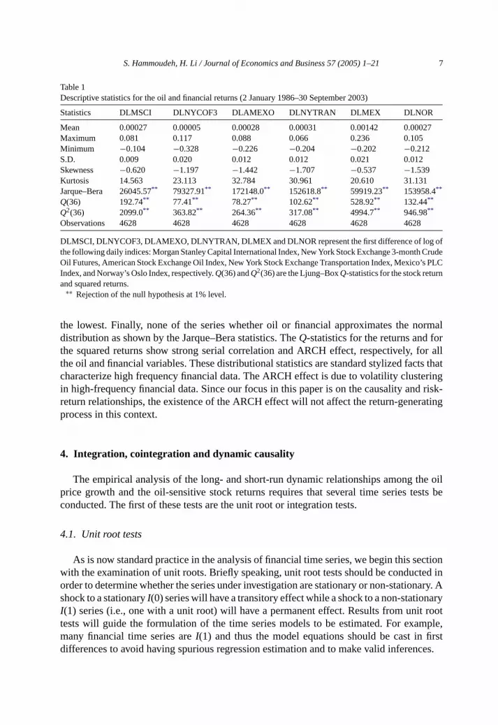
An examination of both the oil and financial returns’ descriptive statistics reveals thatthe Mexican market (MEX) yields the highest daily returns on average over the period 2January 1986–30 September 2003, while the NYMEX 3-month futures oil price (NYCOF3)has the lowest average return (seeTable 1). In terms of daily return volatility over the sameperiod, the Mexican market also has the highest volatility, while the Morgan Stanley CapitalInternational Index (MSCI) has the lowest. Note that the volatilities of the two US specializedindustries, the oil and transportation industries, are close to that of Norway, while that ofthe oil price is close to Mexico’s.
All of the displayed oil and oil-sensitive financial variables in this study have non-symmetric (unconditional) distributions. In terms of skewness the oil price growth, the MSCIreturn and all the oil-sensitive returns are skewed to the left.7 This means that decreases inreturns occur more often than increases.
The major source of non-symmetry of the distributions of the oil and financial returnsin this paper is the excess kurtosis. The kurtosis (K) for all the returns is considerablygreater than 3, indicating that distributions are strongly more leptokurtic than the normaldistribution. Amex Oil has the highest excess kurtosis and the MSCI World Index has
7 Stock returns of other oil-exporting countries such as Indonesia and Russia are skewed to the right.
S. Hammoudeh, H. Li / Journal of Economics and Business 57 (2005) 1–21 7
Table 1Descriptive statistics for the oil and financial returns (2 January 1986–30 September 2003)
DLMSCI, DLNYCOF3, DLAMEXO, DLNYTRAN, DLMEX and DLNOR represent the first difference of log ofthe following daily indices: Morgan Stanley Capital International Index, New York Stock Exchange 3-month CrudeOil Futures, American Stock Exchange Oil Index, New York Stock Exchange Transportation Index, Mexico’s PLCIndex, and Norway’s Oslo Index, respectively.Q(36) andQ2(36) are the Ljung–BoxQ-statistics for the stock returnand squared returns.
∗∗ Rejection of the null hypothesis at 1% level.
the lowest. Finally, none of the series whether oil or financial approximates the normaldistribution as shown by the Jarque–Bera statistics. TheQ-statistics for the returns and forthe squared returns show strong serial correlation and ARCH effect, respectively, for allthe oil and financial variables. These distributional statistics are standard stylized facts thatcharacterize high frequency financial data. The ARCH effect is due to volatility clusteringin high-frequency financial data. Since our focus in this paper is on the causality and risk-return relationships, the existence of the ARCH effect will not affect the return-generatingprocess in this context.
4. Integration, cointegration and dynamic causality
The empirical analysis of the long- and short-run dynamic relationships among the oilprice growth and the oil-sensitive stock returns requires that several time series tests beconducted. The first of these tests are the unit root or integration tests.
4.1. Unit root tests
As is now standard practice in the analysis of financial time series, we begin this sectionwith the examination of unit roots. Briefly speaking, unit root tests should be conducted inorder to determine whether the series under investigation are stationary or non-stationary. Ashock to a stationaryI(0) series will have a transitory effect while a shock to a non-stationaryI(1) series (i.e., one with a unit root) will have a permanent effect. Results from unit roottests will guide the formulation of the time series models to be estimated. For example,many financial time series areI(1) and thus the model equations should be cast in firstdifferences to avoid having spurious regression estimation and to make valid inferences.
8 S. Hammoudeh, H. Li / Journal of Economics and Business 57 (2005) 1–21
The Augmented Dickey–Fuller (ADF) and Perron–Phillips (PP) tests are used in ouranalysis. The results of these tests show that the oil futures price, the two US industryindices and the two national index series for Mexico and Norway in (log of) levels are non-stationary, and are stationary in first differences at the 5% levels (results are not reported inconsideration of space). Therefore, we will conduct the main analysis in terms of petroleumprice growth and stock market returns for the two US industries, Mexico and Norway. Theindividual stochastic trends in the individual non-stationary series may be due to OPECintervention policy, national weather and seasonal variations, business cycle and/or nationalpolitical events in the oil-producing countries and the US.
4.2. Cointegration tests
A system of two or more time series, which are non-stationary in levels and have indi-vidual stochastic trends, can share a common stochastic trend(s). In this case, those seriesare cointegrated. A stationary linear combination of these series is called a cointegratingequation and is considered a cointegrating vector, and may be interpreted as a long-runequilibrium relationship between the variables. In general, the more cointegrating vectorsare in the system, the more stable the system is.8 The presence of cointegration also impliesthat causal or predictive relations in at least one direction exist.
There are many possible tests for cointegration; the most general of them is the mul-tivariate test based on the autoregressive representation discussed inJohansen (1988)andJohansen and Juselius (1990). This paper applies this test to a system of oil and equityreturns, including the world capital market index (MSCI), the NYMEX 3-month futuresprice, the US Amex Oil Index, the US NYSE Transportation Index, Mexico’s PLC In-dex and Norway’s Oslo All Shares Index. This system also encompasses the four trad-ing day dummies (DM for Monday, DT for Tuesday, DW for Wednesday and DR forThursday) relative to Friday and the three economic and political event dummies (D87for the 1987 stock market crash, D90 for the 1990 Gulf war and D97 for the 1997 Asiancrisis).
The cointegration test shows that at the 5% significance level there are three cointegrat-ing vectors (long-run relationships) or equivalently three common stochastic trends amongthe six endogenous variables in this system (Table 2).9 The three common stochastic forcesare related to the global business cycle, the changes in oil price and the occurrence of po-litical events. Based on the significance of the variables in the cointegrating equations and
8 If a five-variable system has, say, four cointegrating vectors (one common trend or one unit root) then thereare four directions where the variance is finite (i.e., stable) and one direction in which the variance is infinite (sincethe variance of a unit root is infinite). If the system has only one cointegrating vector (four common trends or unitroots), then it can deviate in four independent directions and is stable in one direction (Crowder & Wohar, 1998,p. 195).
9 A variant of this system that includes the seven dummies and divides MSCI into an “up market” and “downmarket” was estimated in order to capture the asymmetry in the movements of returns and to avoid the aggregationbias. “Up market” means the MSCI goes up and “down market” means the MSCI goes down. This variant yieldedfour cointegrating vectors. However, contrary to findings in the literature (see for example,Hammoudeh et al.(2003)andPettengill, Sundaram, and Mathur (1995)for the non-oil stock markets), the aggregation bias has nofounding in this system.
S. Hammoudeh, H. Li / Journal of Economics and Business 57 (2005) 1–21 9
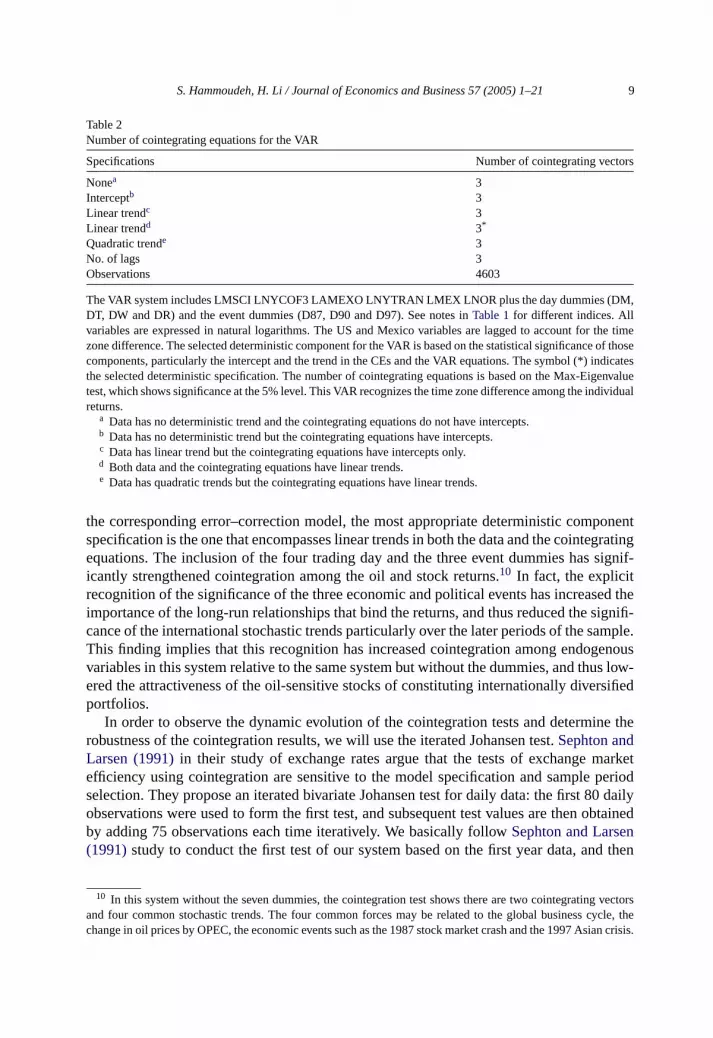
Table 2Number of cointegrating equations for the VAR
The VAR system includes LMSCI LNYCOF3 LAMEXO LNYTRAN LMEX LNOR plus the day dummies (DM,DT, DW and DR) and the event dummies (D87, D90 and D97). See notes inTable 1for different indices. Allvariables are expressed in natural logarithms. The US and Mexico variables are lagged to account for the timezone difference. The selected deterministic component for the VAR is based on the statistical significance of thosecomponents, particularly the intercept and the trend in the CEs and the VAR equations. The symbol (*) indicatesthe selected deterministic specification. The number of cointegrating equations is based on the Max-Eigenvaluetest, which shows significance at the 5% level. This VAR recognizes the time zone difference among the individualreturns.
a Data has no deterministic trend and the cointegrating equations do not have intercepts.b Data has no deterministic trend but the cointegrating equations have intercepts.c Data has linear trend but the cointegrating equations have intercepts only.d Both data and the cointegrating equations have linear trends.e Data has quadratic trends but the cointegrating equations have linear trends.
the corresponding error–correction model, the most appropriate deterministic componentspecification is the one that encompasses linear trends in both the data and the cointegratingequations. The inclusion of the four trading day and the three event dummies has signif-icantly strengthened cointegration among the oil and stock returns.10 In fact, the explicitrecognition of the significance of the three economic and political events has increased theimportance of the long-run relationships that bind the returns, and thus reduced the signifi-cance of the international stochastic trends particularly over the later periods of the sample.This finding implies that this recognition has increased cointegration among endogenousvariables in this system relative to the same system but without the dummies, and thus low-ered the attractiveness of the oil-sensitive stocks of constituting internationally diversifiedportfolios.
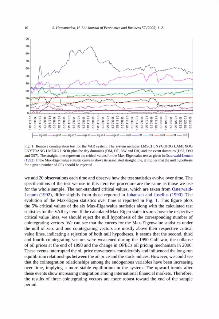
In order to observe the dynamic evolution of the cointegration tests and determine therobustness of the cointegration results, we will use the iterated Johansen test.Sephton andLarsen (1991)in their study of exchange rates argue that the tests of exchange marketefficiency using cointegration are sensitive to the model specification and sample periodselection. They propose an iterated bivariate Johansen test for daily data: the first 80 dailyobservations were used to form the first test, and subsequent test values are then obtainedby adding 75 observations each time iteratively. We basically followSephton and Larsen(1991)study to conduct the first test of our system based on the first year data, and then
10 In this system without the seven dummies, the cointegration test shows there are two cointegrating vectorsand four common stochastic trends. The four common forces may be related to the global business cycle, thechange in oil prices by OPEC, the economic events such as the 1987 stock market crash and the 1997 Asian crisis.
10 S. Hammoudeh, H. Li / Journal of Economics and Business 57 (2005) 1–21
Fig. 1. Iterative cointegration test for the VAR system. The system includes LMSCI LNYCOF3G LAMEXOGLNYTRANG LMEXG LNOR plus the day dummies (DM, DT, DW and DR) and the event dummies (D87, D90and D97). The straight lines represent the critical values for the Max-Eigenvalue test as given inOsterwald-Lenum(1992). If the Max-Eigenvalue statistic curve is above its associated straight line, it implies that the null hypothesisfor a given number of CEs should be rejected.
we add 20 observations each time and observe how the test statistics evolve over time. Thespecifications of the test we use in this iterative procedure are the same as those we usefor the whole sample. The non-standard critical values, which are taken fromOsterwald-Lenum (1992), differ slightly from those reported inJohansen and Juselius (1990). Theevolution of the Max-Eigen statistics over time is reported inFig. 1. This figure plotsthe 5% critical values of the six Max-Eigenvalue statistics along with the calculated teststatistics for the VAR system. If the calculated Max-Eigen statistics are above the respectivecritical value lines, we should reject the null hypothesis of the corresponding number ofcointegrating vectors. We can see that the curves for the Max-Eigenvalue statistics underthe null of zero and one cointegrating vectors are mostly above their respective criticalvalue lines, indicating a rejection of both null hypotheses. It seems that the second, thirdand fourth cointegrating vectors were weakened during the 1990 Gulf war, the collapseof oil prices at the end of 1998 and the change in OPECs oil pricing mechanism in 2000.These events interrupted the oil price movements considerably and influenced the long-runequilibrium relationships between the oil price and the stock indices. However, we could seethat the cointegration relationships among the endogenous variables have been increasingover time, implying a more stable equilibrium in the system. The upward trends afterthese events show increasing integration among international financial markets. Therefore,the results of three cointegrating vectors are more robust toward the end of the sampleperiod.
S. Hammoudeh, H. Li / Journal of Economics and Business 57 (2005) 1–21 11
4.3. Causality in the vector error–correction models
If a set of non-stationary variables is cointegrated, then an unrestricted vector auto-regression model (VAR) comprised of the first differences of these variables alone will bemisspecified, and information on long-term equilibrium relationships among the variableswill be lost. In this case it is appropriate to use the vector error–correction (VEC) model.This model can be specified by the following set of equations:
where DLV are first differences of the vector [MSCI, NYCOF3, AMEXO, NYTRAN, MEX,NOR]′ andε is a vector of the residuals. This model includes three error–correction terms(ECT1, ECT2, ECT3) that represent deviations from the long-run equilibrium, the fourtrading day dummies for Monday, Tuesday, Wednesday and Thursday (DM, DT, DW andDR, respectively) and the three event dummies (D87, D90 and D97). The dummy variablesare included to account for the day-of-the-week effect, and the event dummies are meantto capture the major political and financial events that took place during the sample period.The model also allows for interpretation of the adjustment process following a state ofdisequilibrium by including the lagged dependent variables (DLVt−j). The lag lengthk isdetermined by the AIC criterion, i.e.,k= 4.
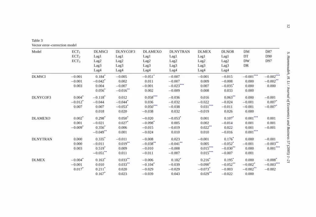
The estimates of the oil-based, six variable VEC model are reported inTable 3. Theseestimates suggest that on a daily basis there is a negative bi-directional dynamic relationshipbetween the oil futures price growth and the return of the world capital market as representedby MSCI, with the latter having the stronger impact (4-day cumulative effect of−0.137from DLMSCI to DLNYCOF3 versus−0.026 from DLNYCOF3 to DLMSCI). This resultimplies that that MSCI returns and NYCOF3 growth can be used to predict each other on adaily basis. The significant coefficient estimates of lagged DLNYCOF3 in each equation inthe system also point out that on a daily basis the oil price growth leads the individual stockreturns of all the oil-exporting countries and the oil-sensitive industries, as well as the worldcapital market’s return in the standard aggregate mode. The oil price lead impact is positiveon all the oil-sensitive returns but is negative on the world capital market’ return whichresponds laggardly to this impact. In comparison to the oil price lead, the world capitalmarket’s return has much stronger positive impact on all the individual stock returns, asshown in the third column ofTable 3. This result is a strong indication that these oil-sensitivestock markets are well integrated with the world stock markets and the systematic risk hasgreater influence than the oil price sensitivity. Still it will be interesting to examine the oilprice growth and the world capital market’s lead impacts in up and down markets. Thisinterest should pave the way for our second follow-up approach in using factor models totestHypothesis 2.
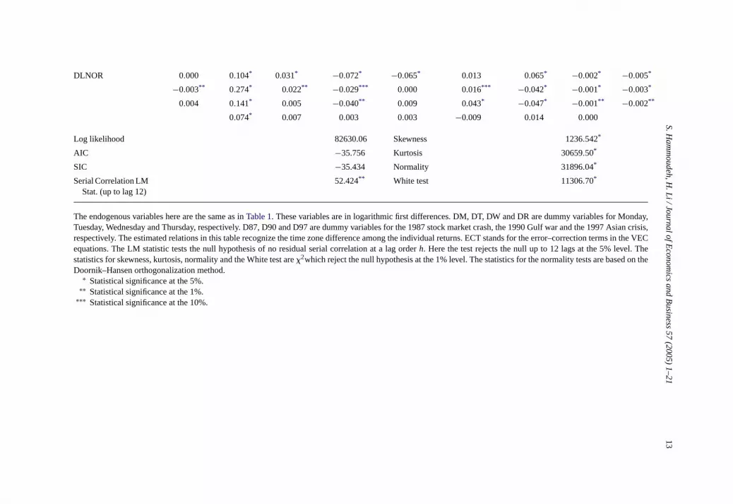
As expected, the US oil industry return is the most positively and dynamically sensitiveto changes in the oil price, displaying no corrections for two consecutive days. Mexico andNorway also show similar sensitivity patterns to the oil price change. On the other hand,
The endogenous variables here are the same as inTable 1. These variables are in logarithmic first differences. DM, DT, DW and DR are dummy variables for Monday,Tuesday, Wednesday and Thursday, respectively. D87, D90 and D97 are dummy variables for the 1987 stock market crash, the 1990 Gulf war and the 1997 Asian crisis,respectively. The estimated relations in this table recognize the time zone difference among the individual returns. ECT stands for the error–correction terms in the VECequations. The LM statistic tests the null hypothesis of no residual serial correlation at a lag orderh. Here the test rejects the null up to 12 lags at the 5% level. Thestatistics for skewness, kurtosis, normality and the White test are�2which reject the null hypothesis at the 1% level. The statistics for the normality tests are based on theDoornik–Hansen orthogonalization method.
∗ Statistical significance at the 5%.∗∗ Statistical significance at the 1%.
∗∗∗ Statistical significance at the 10%.
14 S. Hammoudeh, H. Li / Journal of Economics and Business 57 (2005) 1–21
only Norway and the world market index have a 1 day lead relationship with the oil price atthe 5% significance level, with Norway having a positive lead and MSCI having a negativelead.11
Comparing the lead–lag relationships between the returns of the oil-exporting countriesand those of the US oil-sensitive industries, the results suggest that increases in the USindustries’ returns lead, for the most part, to negative changes in the returns of the oil-exporting countries. On the other hand, increases in the returns of the oil-exporting countrieslead to increases in the returns of the US industries. This implies that investors in a risingmarket should first invest in the stocks of the oil-exporting countries and then move intothe stocks of the two US oil-sensitive industries.
In terms of the effects of the dummies on the daily dynamic relationships relative toFriday, there is no distinct pattern of sensitivity for the trading day effect for all the industryand country indices. Among all the returns considered, Norway stands out as the mostsensitive to the Monday, Tuesday and Wednesday trading day dummies. It is possible thatNorway’s All-Shares exhibits an extended negative week-end effect and digests informationmore slowly than the American markets, and it also responds to weekly domestic and foreigneconomic releases because of the presence of foreign capitalization in the market. However,those country and industry returns are more sensitive to the political and economic dummies.The world capital market as represented by MSCI shows negative sensitivity to the 1987stock market crash and the 1990 Gulf war, which was followed by a recession in the US.The US transportation industry and the oil price were affected by both the 1990 Gulf warand the 1997 Asian crisis which led to the collapse of the oil price in 1998, Mexico by the1987 stock market crash and the 1990 Gulf war, and Norway by all three event dummies.It should not be a surprise that the MSCI shows negative sensitivity to the collapse of theworld stock markets in 1987. The transportation industry’s negative response to the 1990Gulf war is a mixture of sensitivities to higher oil prices and terrorist threats at that timeparticularly to those directed at the US airline industry. Moreover, its weak but positiveresponse to the 1997 Asian crisis could be due to the collapse of oil prices in 1998. Norway,as both a diversified and oil-based economy and whose stock index is an all-share, seemsto be negatively sensitive to all kinds of oil, economic and political dummies. The lack ofsensitivity of the US oil industry return to the three events is perhaps due to its being directlyand strongly sensitive to the changes in the oil price, which itself was directly affected byall those events. Thus, the indirect link of this industry to the event dummies gave rise toits muted (or lack of) response. Moreover, it is possible that those event dummies do notaffect the US oil industry on a daily basis.
In this VEC system all the variables except MSCI and Norway enter the cointegratingequations significantly, which implies that those variables participate in forming long-runrelationships, whereas MSCI and Norway do not (seeTable 4). It is possible that becauseMSCI is a composite stock index that includes more than 40 national stock markets and thatit leads the oil price, this index’s return enters the system indirectly and through both the oilprice change and the four oil-sensitive stock markets’ returns. Additionally, it is possiblethat MSCI may not participate in long-run relationships with all the other variables on adaily basis. Although Norway is an oil-based country, its economy and its stock index are
11 Amex oil has a 1 day positive lead at the 10% significance level.
S. Hammoudeh, H. Li / Journal of Economics and Business 57 (2005) 1–21 15
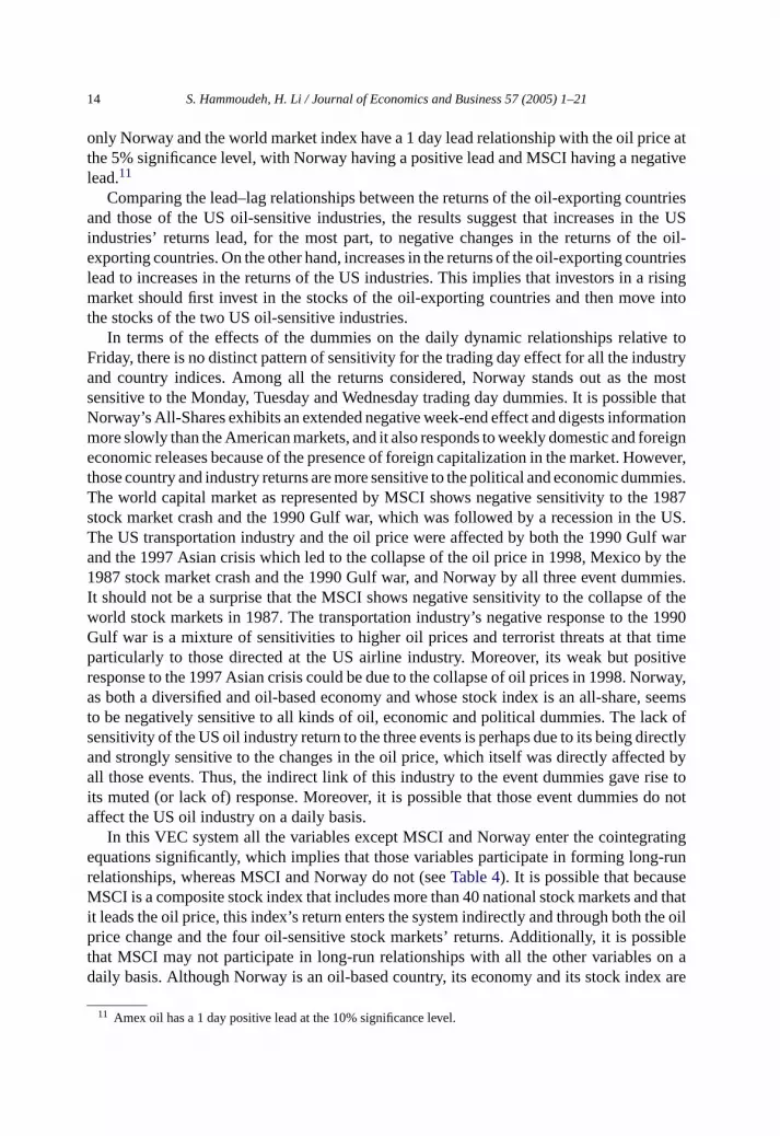
Table 4Significance of zero restrictions on coefficients of cointegrated equations of the VEC model
See notes inTable 1for the explanation of variables, which are in logarithmic forms in this table. Therefore, inthis VAR system with dummy variables, LMSCI and LNOR do not form long-run equilibrium relationships withother returns in this system.
∗ The LR tests reject the null hypothesis that theith endogenous variable does not enter the cointegratingequations significantly at the 5% level.
∗∗ The LR tests reject the null hypothesis that theith endogenous variable does not enter the cointegratingequations significantly at the 1% level.∗∗∗ The LR tests reject the null hypothesis that theith endogenous variable does not enter the cointegratingequations significantly at the 10% level.
more diversified than the other oil-sensitive indices considered in this system. Its index isalso an all-share index with no oil capitalization but it includes significant foreign stockcapitalization and entertains signals from foreign markets.
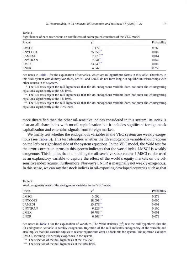
We finally test whether the endogenous variables in the VEC system are weakly exoge-nous (seeTable 5). This test identifies whether theith endogenous variable should appearon the left- or right-hand side of the system equations. In the VEC model, the Wald test forthe error–correction terms in this system indicates that the world index LMSCI is weaklyexogenous. This implies that in modeling the oil-sensitive stock returns LMSCI can be usedas an explanatory variable to capture the effect of the world’s equity markets on the oil-sensitive index returns. Furthermore, Norway’s LNOR is marginally not weakly exogenous.In this sense, we can say that stock indices in oil-exporting developed countries such as that
Table 5Weak exogeneity tests of the endogenous variables in the VEC model
See notes inTable 1for the explanation of variables. The Wald statistics (χ2) test the null hypothesis that theith endogenous variable is weakly exogenous. Rejection of the null indicates endogeneity of the variable andalso implies that this variable adjusts to restore equilibrium after a shock hits the system. The rejection excludesLMSCI, meaning it is weakly exogenous in the system.
∗∗ The rejection of the null hypothesis at the 1% level.∗∗∗ The rejection of the null hypothesis at the 10% level.
16 S. Hammoudeh, H. Li / Journal of Economics and Business 57 (2005) 1–21
of Norway have more explanatory power in determining the movements of oil prices and theoil-sensitive stock indices than those of oil-exporting developing countries such as Mexicowhose index is dominated by shares of companies engaged mainly in telecommunication,construction and supermarkets.12
5. Risk and equity returns
The oil futures price and MSCI in the dynamic, simultaneous VAR are found to besignificant and lead the oil-sensitive stock returns individually in a group and also formlong-run relationships with them. We wish to further investigate the roles of these twofactors within an international arbitrage price theory (APT) framework in the standardaggregate model and in the up and down models which are specified in relation to the worldcapital market. Thus, the purpose is to compare the sensitivity of stock returns to changes inthe global factors with their sensitivity to the oil price. We also wish to test whether or notasymmetry in return sensitivity exists when the world capital market is in an up and downmodes. All these considerations complement the results derived in Section4 from the VECmodel, which is usually not suited for such analysis. In the international APT model, weestimate the industry and country systematic risks (betas) with respect to the world capitalmarket (MSCI) while controlling for oil sensitivity as represented by NYMEX 3-monthfutures price. This approach also allows for asymmetry to be taken explicitly into accountand it thus complements the VAR approach. The investment risk or beta examined in theAPT approach is relevant for traders and managers of international stock portfolios becauseit is usually priced in return compensations.
The following general equation captures the industry or country’s risk in a standardmarket:
where DLYj is the daily return for the industry or country stock index, DLMSCI the MorganStanley Capital Market Index and DLNYCOF3 the daily oil price growth for the NYMEX 3-month futures price.13 The equation is estimated using OLS with White heteroskedasticity-consistent covariance. In Eq.(2), β1j is called theunconditionalsystematic risk becausethis measure of risk is not different no matter in which direction the world market MSCImoves. A positive (negative)β1j implies a positive (negative) association between the dailymovement of thejth industry or country market and that of the world capital market.
However, investment risk may have different behavior depending on whether the worldcapital market is up (down) and the return is positive (negative) for the same time periodunder consideration. Many studies have shown that the unconditional systematic risk (betas)and returns may not be related empirically due to the bias created by the combination
12 Hammoudeh and Eleisa (2004)found in an oil price-based system that includes Bahrain, Kuwait, Oman,Saudi Arabia and UAE stock markets as well as an oil futures price, only the Saudi market has a predictive powerfor future movements of the oil futures price.
13 The correlation between DLNYCOF3 and DLMSCI is very low and stands at−0.045, so there is no multi-collinearity problem in this equation.
S. Hammoudeh, H. Li / Journal of Economics and Business 57 (2005) 1–21 17
of positive and negative returns (see for example,Fletcher, 2000; Tang & Shum, 2003;Hammoudeh, Ewing, & Zhao, 2003). Therefore, as suggested byPettengill, Sundaram, andMathur (1995), those returns should be segregated. Taking into account this asymmetry,Eq.(2) can be rewritten as
DLY jt = β0j + β+1j × du× DLMSCIt + β−
1j(1 − du)
× DLMSCIt + γ1j DLNYCOF3t + ejt (3)
where du is the dummy variable that takes on the value of one for the world’ up market,that is, when DLMSCI > 0, and takes on the value of 0 for its down market (i.e., whenDLMSCI < 0). In Eq.(3), β+
1j is thejth industry/country’s conditional systematic risk when
this market is up andβ−1j is jth industry/country’s conditional systematic risk when the
market is down. Basically, the world return series DLMSCI is divided into two series,one with positive numbers for the up market and the other with negative numbers for thedown market. The dummy du creates the positive return series and (1− du) establishes thenegative return series.
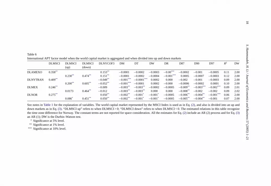
Table 6reports the sensitivities of the oil-sensitive stock returns of the two US oil-sensitive industries (oil and transportation) and the two oil-based countries (Mexico andNorway) to both the oil price growth and MSCI return in the cases of the world’s stan-dard market and its up and down markets as specified in Eqs.(2) and (3), respectively.These results for both equations are consistent with those derived from the VEC modelin Table 3. Although all the countries and the industries are strongly oil price-based, theestimates suggest that the (systematic) risk associated with the world capital market returnoverwhelmingly dominates the sensitivity to the oil price change. This finding is consistentwith the results of the VEC model as shown inTable 3. Moreover, the estimates of theunconditional and unconditional industry/country betas are significant for all the countriesand industries in the cases of the standard world market, and the up and down markets withthe exception of the Mexican return in the up market. The US transportation industry hasthe greatest investment systematic risk (beta) in the standard and the down markets, whilethe US oil industry has the greatest risk in the up market. Relating the estimates of thesystematic risk in Eq.(2) of the standard market to those of standard deviation inTable 1,one can infer that the unsystematic (idiosyncratic) risks for the two US industries are lowerthan those for Norway and Mexico. A possible explanation for Mexico is that its indexhas only 36 stocks which are dominated by the shares of companies engaged mainly intelecommunication, construction and supermarkets Another possible reason for this coun-try, having both the highest standard deviation (total risk) and unsystematic risk, is that thiscountry is an emerging economy that has faced major financial and political risks and is stillsusceptible to future political and economic crises. Policy implication in this case is thatinvestors should hold Mexican, and to some extent Norwegian, stocks in internationallydiversified portfolios in order to diversify away the high unsystematic risk.
The Wald test suggests that estimated conditional beta in Eq.(3)is not symmetric betweenthe world’s up and down markets for all the industry/country returns, with the down marketrisk being considerably greater than that of the up market (test results are available uponrequest).
18S.H
ammoudeh,H
.Li/Jo
urnalofE
conomics
andBusin
ess
57(2005)1–21
Table 6International APT factor model when the world capital market is aggregated and when divided into up and down markets
See notes inTable 1for the explanation of variables. The world capital market represented by the MSCI Index is used as in Eq.(2), and also is divided into an up anddown markets as in Eq.(3). “DLMSCI up” refers to when DLMSCI > 0; “DLMSCI down” refers to when DLMSCI < 0. The estimated relations in this table recognizethe time zone difference for Norway. The constant terms are not reported for space consideration. All the estimates for Eq.(2) include an AR (2) process and for Eq.(3)an AR (1); DW is the Durbin–Watson test.
∗ Significance at 5% level.∗∗ Significance at 1% level.
∗∗∗ Significance at 10% level.
S. Hammoudeh, H. Li / Journal of Economics and Business 57 (2005) 1–21 19
The findings ofTable 6imply that aggressive investors and aggressive growth portfoliomanagers interested in oil-sensitive stocks with higher returns may be inclined to buy stocksthat belong to industries or countries with higher beta, such as the US oil and transportationindustries. However, they should be willing to accept abnormal losses in the down market ifthey invest in those markets, particularly in the transportation industry. Risk-averse investorsand balanced portfolio managers should invest in stocks of sectors with relatively lower betasuch as Norway.
The estimates of the above equations also suggest that oil price growth is priced in thereturns or compensations demanded by the investors in these markets. The oil sensitivity ispositive in the cases of the US Amex Oil Index and the Norway Oslo All-Shares Index butnegative in the cases of the US Transportation Index. The oil price sensitivity does not seemto be significant in the case of Mexico perhaps because of this country’s repeated majordomestic economic and political crises. Another reason is that Mexico’s index is dominatedby securities in the telecommunication, construction and super markets which are not thatoil sensitive.
In terms of the effects of the trading day dummies, the estimates seem to suggest that mostof the returns display the negative week-end effect on Monday returns, and the exceptionis the US oil industry. The other trading days do not have consistently significant effectsacross the returns as is the case in the VEC model. In term of the event dummy effects, the1987 world stock market crash and the 1990 Gulf war, which affected major oil-exportingcountries and was accompanied by a recession in the US, have the most significant impactwhich is also consistent with the findings of the VEC model. The 1997 Asian crisis affectedMexico.
6. Conclusions
These estimates suggest that on a daily basis there is a negative bi-directional dynamicrelationship between the oil futures price growth and the return of the world capital marketas represented by MSCI, with the latter having the stronger impact. This result meansthat higher oil prices are bad for the world capital market as a whole. The internationalAPT model also confirms this result, regardless whether the world capital market is upor down. This finding implies that MSCI returns and NYCOF3 growth can be used topredict each other on a daily basis. Moreover, since those two variables move in differentdirections, the MSCI index and the NYMEX 3-month futures contracts can be combinedin an international portfolio to diversify away unsystematic risk. In contrast, the findingssuggest that the oil price growth has a positive impact on the oil-related stocks. Thus, thesestocks in combination with the other stocks in MSCI are good candidates to diversify awayidiosyncratic risk.
At the individual country and industry levels, both the MSCI returns and NYCOF3 growthlead all the individual oil-sensitive returns considered in this study, with MSCI having thestronger impact. This result suggests that those oil-sensitive markets are well integratedwith the world capital market. Based on the extent of returns’ positive dynamic sensitivityto oil price growth, in a rising oil market investors interested in those oil-sensitive stocksshould invest first in the stocks of the US oil industry and then in the Mexican stocks before
20 S. Hammoudeh, H. Li / Journal of Economics and Business 57 (2005) 1–21
they invest in the Norwegian stock to take advantage of higher oil prices.14 Contrary to theresults of the VEC model, the APT model found a negative relationship between the UStransportation industry and the oil price, making the stocks of this cyclical industry to becontrarians to those of the stocks of the other markets examined in this article. In the caseof rising world capital market, investors should also invest first in the US oil industry, thenin the US transportation industry, Norway and Mexico which is dominated by supermarket,construction and telecommunication stocks.
For the prediction of the oil price, only Norway and the world market index have alead relationship with the oil price, with Norway having a positive 1 day lead and MSCIhaving a negative 1 day lead. In the case of the five GCC oil-exporting countries studiedby Hammoudeh and Eleisa (2004), only Saudi Arabia has a predictive power of the oilprice. These conclusions imply that not all stock markets of the oil-exporting countries andoil-sensitive industries can predict the futures oil price on a daily basis.
In terms of the dummies in the presence of daily dynamic relationships Norway, andto some extent Mexico, seems to display the most sensitivity to the trading day, politicaland economic event dummies. Therefore, although these countries’ stock returns displayrelatively strong dynamic sensitivity to oil price growth, they can be marred by the tradingday and event effects. The oil price is affected by the events related to the oil-exportingcountries such as the 1990 Gulf war and the 1997 Asian crisis. The Asian countries arethe most growing source of demand for the Gulf oil. Unsurprisingly, the world capitalmarket showed negative dynamic sensitivity to the 1987 stock market crash and the 1990Gulf war.
In terms of the univariate relationships between risks and returns in the factor model,the size of the systematic risk is greater than that of oil price growth impact for these oil-sensitive stock indices regardless of the direction of the world capital market. This resultthus implies that investors view the world market return as a more significant factor inpricing those oil-sensitive returns than the oil price growth.
Acknowledgements
The authors wish to thank the editors Kenneth Kopecky and Ravi Shukla, and two anony-mous referees for careful reading and valuable comments on an earlier draft of this article.They also thank Jennifer Weber of Morgan Stanley Capital International for providing thedata on the MSCI World Index.
References
Bekaert, G., & Harvey, C. F. (1995). Time-varying world market integration.Journal of Finance, 50(2), 403–444.Crowder, W. J., & Wohar, M. E. (1998). Cointegration, forecasting and international stock prices.Global Finance
Journal, 9(2), 181–204.
14 This result is based on summing up the significant estimated coefficients of the endogenous variables.
S. Hammoudeh, H. Li / Journal of Economics and Business 57 (2005) 1–21 21
Ferson, W. E., & Harvey, C. R. (1994). Sources of risk and expected returns in global equity markets.Journal ofBanking and Finance, 18(4), 775–803.
Fletcher, J. (2000). On the conditional relationship between beta and return in international stock returns.Inter-national Review of Financial Analysis, 9, 235–245.
Hammoudeh, S., & Eleisa, L. (2004). Dynamic relationships among GCC stock markets and NYMEX oil futures.Contemporary Economic Policy, 22(2), 250–269.
Hammoudeh, S., Ewing, B., & Zhao, G. (2003). Oil and natural gas sensitivity, asymmetry, systematic risk andskewness in the Russian stock market. Working Paper. Drexel University.
Hammoudeh, S., & Li, H. (2004). The impact of the Asian crisis on the behavior of US and international petroleumprices.Energy Economics, 26, 135–160.
Heston, S. L., Rouwenhorst, K. G., & Wessels, R. E. (1995). The structure of international stock returns and theintegration of capital markets.Journal of Empirical Finance, 2(3), 173–197.
Huang, R., Masulis, R., & Stoll, H. (1996). Energy shocks and financial markets.Journal of Futures Markets,16(10), 1–27.
Johansen, S. (1988). Statistical analysis of cointegration vectors.Journal of Economic Dynamics and Control, 12,231–254.
Johansen, S., & Juselius, K. (1990). Maximum likelihood estimation and inferences on cointegration-with appli-cations to demand for money.Oxford Bulletin of Economics and Statistics, 52, 169–210.
Jones, C., & Kaul, G. (1996). Oil and stock markets.Journal of Finance, 51(2), 463–491.Karolyi, A. G., & Stultz, R. M. (2003). Are financial assets priced locally or globally? In D. Constantinides, M.
Harri, & R. M. Stulz (Eds.),Handbook of the economics of finance. Amsterdam: North-Holland.Osterwald-Lenum, M. (1992). A note with quintiles of the asymptotic distribution of the maximum likelihood
cointegration rank statistics.Oxford Bulletin of Economics and Statistics, 54, 46–472.Pettengill, G. N., Sundaram, S., & Mathur, I. (1995). The conditional relations between beta and returns.Journal
of Financial and Quantitative Analysis, 30, 101–116.Sadorsky, P. (1999). Oil price shocks and stock market activity.Energy Economics, 21, 449–469.Sephton, P., & Larsen, H. (1991). Tests of exchange market efficiency: fragile evidence from cointegration tests.
Journal of International Money and Finance, 10, 561–570.Tang, G., & Shum, W. (2003). The relationships between unsystematic risk, skewness and stock reruns during up
and down markets.International Business Review, 12, 523–541.