Vol. 118 (2010) ACTA PHYSICA POLONICA A No. 4

Modern Rheology on a Stock Market:Fractional Dynamics of Indices

M. Kozłowska and R. KutnerDivision of Physics Education, Institute of Experimental Physics, Department of Physics, Warsaw University

Smyczkowa Str. 5/7, PL-02-678 Warsaw, Poland

(Received January 29, 2010)

This paper presents an exactly solvable (by applying the fractional calculus) the rheological model offractional dynamics of financial market conformed to the principle of no arbitrage present on financial market. Therheological model of fractional dynamics of financial market describes some singular, empirical, speculative dailypeaks of stock market indices, which define crashes as a kind of phase transition. In the frame of the model theplastic market hypothesis and financial uncertainty principle were formulated, which proposed possible scenariosof some market crashes. The brief presentation of the model was made in our earlier work (and references therein).The rheological model of fractional dynamics of financial market is a deterministic model and it is complementaryto already existing other ones; together with them it offers possibility for thorough and widespread technicalanalysis of crashes. The constitutive, fractional integral equation of the model is an analogy of the correspondingone, which defines the fractional Zener model of plastic material. The fractional Zener model is the canonical onefor modern rheology, polymer physics and biophysics concerning non-Debye relaxation of viscoelastic biopolymers.The useful approximate solution of the constitutive equation of the rheological model of fractional dynamics offinancial market consists of two parts: (i) the first one connected with long-term memory present in the system,which is proportional to the generalized exponential function defined by the Mittag–Leffler function and (ii) thesecond one describing oscillations (e.g. beats or oscillations having two slightly shifted frequences). The shapeexponent leading the Mittag–Leffler function, defines here the order of the phase transition between bullish andbearish states of the financial market, in particular, for recent hossa and bessa on some small, middle and largestock markets. It happened that this solution also successfully estimated some long-term price dynamics on thehypothetical market in United States.

PACS numbers: 89.20.−a, 89.65.−s, 89.65.Gh, 89.90.+n

1. Introduction

The bubbles and crashes are considered as unavoid-able elements of stock market dynamics. They play akey role for capitalistic, competitive free markets [1–4, 5].Therefore bubbles and crashes are the natural subject ofthorough and widespread studies of economists, sociolo-gists, psychologists and recently, econo- and sociophysi-cists. The most fruitful seems to be the concept of thediscrete scale invariance applied to stock markets andconsidering their crashes as a kind of criticality. As aconsequence the dynamics of the market within the scal-ing region (i.e. in the region preceding a crash) can bedescribed by scale-free laws containing logarithmic pe-riodicities [6–16] (and references therein). The majorachievement of the approach makes possible a forecastingof crash times.

There are many other fruitful analogies between thedynamics and/or stochastics of complex physical and eco-nomical or even social systems [17–25]. The methodsand algorithms that have been explored for describingphysical phenomena become an effective background andinspiration for very productive methods and algorithmsused in analysis of economical, in particular the financialempirical data [16, 26].

Our concept is to consider only well developed tempo-ral, non-exponential, speculative peaks of stock marketindices. It relates in some sense to the idea of Eliezer andKogan [9] (and references therein), which distinguishesthe dynamics of the market in a crashing phase, fromthe one in the quiescent phase. In real market tradersmay form groups which then share information and actin coordination. This is the result of mutual interactionbetween traders leading to herding; groups may tradewith each other through some centralized market proce-dure. We take into consideration the herding effect byway complementary to the approach already developedby percolation models [5, 27].

The solution supplied by our rheological model of thefractional dynamics of financial market (RMFDFM) iscomplementary to the power-law superposed with log--periodic oscillations [2, 16]. We applied it here to de-scribe some empirical data proceeding a crash, whichcannot be successfully handled by the latter approach.Both approaches can constitute together a solid base forforecasting burdened with reduced risk.

The analysis was supported by the non-Debye ornon-exponential relaxation processes observed in stress--strain relaxation of viscoelastic materials [28–33] as well

(677)

678 M. Kozłowska, R. Kutner

as in the tick-by-tick empirical data for FUND futurecontract prices traded at LIFFE London [34].

In this paper we study, by way of examples, some men-tioned above peaks and concern recent hossa and bessa:

(i) on emerging market: the daily closings of the his-torical Warsaw Stock Exchange (WSE) index WIG.We can assume that the dynamics of the WSE istypical for an emerging financial market of smallsize.

(ii) Besides, we study the Deutscher Aktien Index(DAX) as the index typical for middle stock mar-kets and

(iii) Down Jones Industrial Average (DJIA) and SCI∗indices as representative ones for large stock mar-kets.

2. Non-Debye relaxation

It is important to know that the non-Debye relaxationmay arise from memory, i.e. the underlying fundamentalprocesses are of non-Markovian type. It was shown thatfractional calculus is quite natural way of incorporatingmemory effects. The power-law kernel defining the frac-tional relaxation equation presents a long-term memory.The function that plays a dominating role in fractionalrelaxation problems is the Mittag–Leffler (ML) function[31]:

Eα

(−

( | tc − t |τ

)α)=

∞∑n=0

[−(| tc − t | /τ)α]n

Γ (1 + αn),

α > 0 , (2.1)which is a straightforward generalisation of the exponen-tial one (obtained for α = 1) and complementary to thefamous Tsallis q-exponent [3] (here t is time and tc is thelocalization of the turning point from raising to fallingparts of the ML function while α is the shape exponent).The ML function allows interpolation [1] between the cor-responding stretched exponential function for short-timelimit and power-law decay for asymptotic time (whenα < 1); the former plays a crucial role in our analysis.

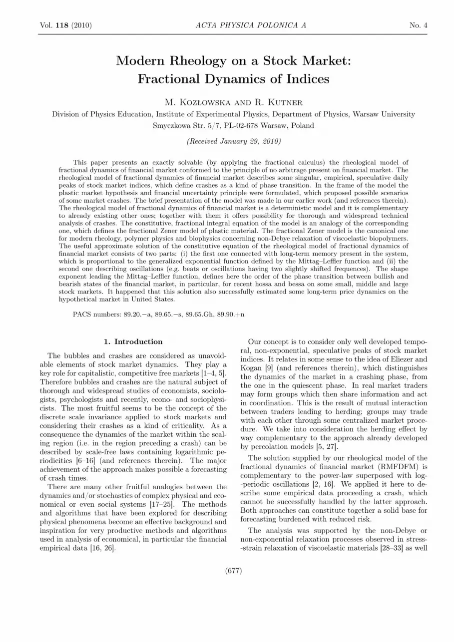
Before we go to financial markets, we pay our atten-tion, for example, to the market of houses and parcelsin U.S. As it is seen in Fig. 1, empirical data proceed-ing from this market is well fitted by the Mittag–Lefflerfunction (red curve) even near to the turning point (i.e.to the point where hossa changes to bessa). The valuesof parameters of ML function obtained here are as fol-lows: the localization of the turning point (maximum) isat tc = 231 months, i.e. at March’07, which is placed ex-actly at the maximum of empirical data, the relaxation

∗ We chose Shanghai Composite Index intead of the Nikkei indexas the latter too much oscillates.

time τ = 95 months, the shape parameter α = 0.60.Let us note that for α < 1 both derivatives (i.e. left- andright-sided) of the ML function diverges at tc according tothe power law, which means that return also accordinglydiverges [1]. Hence, at tc we deal with analogy of thefirst order phase transition. The corresponding predic-tions of exponential function (green curve) and stretchedexponential one (blue curve) were also shown there forcomparison†.

Fig. 1. The median, S, of prices of houses andparcels sold in U.S. between January 1988 and De-cember 2008 (the unit of timescale is chosen here asone trading month). The empirical data (markedby dots) were downloaded from the internet addresshttp://www.economagic.com/ (solid curves were de-fined in the main text).

Quite often the ML function appears both in thestochastic and deterministic modelling of disordered sys-tems. The canonical example of the former may be thecontinuous-time random walk model (CTRW) used in thecontext of a financial market (Refs. [23–34, 35], while thelatter — already mentioned above fractional relaxationequation describing relaxation of viscoelastic materials.

3. Rheological model of fractional dynamicsof financial market

Presentation of our phenomenological, deterministicRMFDFM consists of two stages:

(i) Formulation of a linear ordinary differential equa-tion (LODE) of the first order; this equation de-scribes the index relaxation on an ideal market(considered in Sect. 3.1), i.e. only the exponentialrelaxation of an auxiliary index. By term “relax-ation” we understand here and below in the textthe relaxation both in forward and backward time--directions (of course, this backward relaxation ofthe index is equivalent to its increase in forwardtime-direction).

† For both exponential and stretched exponential functions relax-ation time is given here by τ [Γ (1 + α)]1/α = 79 months.

Modern Rheology on a Stock Market . . . 679

(ii) Fractional generalization of the LODE by using thereplacing transformation that changes the abovementioned differential equation to a more generalfractional form (including, by definition, the long--term memory). Thus we are able to model thenon-exponential (non-Debye) relaxation of the em-pirical index on a real market within the range ofspeculative peaks. For example, the left path of thepeak can initially increase very slowly and acceler-ates strongly toward the end of the peak, formingsingularity of the first order‡. The right paths canhave an opposite dependence on time, i.e. initiallyrapidly decreases and finally very slowly. Of course,we also consider singularities of higher orders.

These stages define the general strategy, which wassupplied by physical papers [28–30, 36–38] concerningrheological problems. The strategy was used for descrip-tion of the non-Debye relaxation of viscoelastic mate-rials and constitutes the basis for developing the frac-tional solid model (FSM). There are several versions ofFSM [28] based on the so-called “fractional elements” de-fined by different mechanical arrangements of springs (i.e.elastic elements) and dashpots (i.e. friction ones), whichare their fundamental structural quants. Such arrange-ment defines the rheological (macroscopic) properties ofa solid, however several different arrangements can definethe same properties.

The RMFDFM considers spring–dashpot pair as ananalog of a single trader (investor), where spring symbol-izes trader’s activity and dashpot his aversion to risk§. Ifspring is stretched it means that investor buys stocks,if it is contracted then stockes are sold, otherwise (whenspring leaves unchanged) the trader is waiting (or is doingnothing). The dashpot always acts (due to the friction oraversion to any risk) against any trader’s activity. Hence,arrangement of spring–dashpot pairs defines a networkof investors, which forms a social cooperative structurefor a given stock market. The model is related to fieldcalled behavioural finance since it somehow incorporatesthe psychological motivation of investor’s behaviour.

In our case the transition from stage (i) to stage (ii)means that the system under considerations changes froman ideal and unrealistic one to a realistic, complex sys-tem, where memory plays an essential role. This mem-ory is defined by the integral, long-term kernel, analo-gously as it was done in terms of the FSM (cf. Eq. (3.13)in Sect. 3.3). By using our approach we describedwell developed speculative peaks concerning recent bessaand hossa present on small, middle and large financialmarkets.

‡ We say the function has singularity of n-th order at given pointif its n-th order derivative diverges at this point but ones of alllower orders do not.

§ This definition of trader does not exclude pathological possibil-ities that only the spring or only the dashpot represent sometrader.

3.1. Evolution of the auxiliary index

The considerations given in this section (in particular,concerning Eq. (3.11)) realize at the present the stage(i) (defined at the beginning of Sect. 3), i.e. the idealstock market dynamics (relaxation) for given path of thespeculative peak.3.1.1. Basic assumptions of the model

The RMFDFM is based on the following fundamentalassumptions:

A1) In the range of well-defined speculative peaks (con-sisting of hossa and bessa paths), the dominating be-haviour of the stock market results from traders’ activi-ties whose strategies are based only on a direct (on-line)observation of the market state. They are conductinga technical analysis of dynamics of stock market indicesand the volume of the corresponding assets and under-take decision. They are called technical traders, chartistsor noise traders. Of course, traders can mutually com-municate without any delay (e.g. by using phones) andexchange informations.

The reason why technical traders dominate the stockmarket within the range of speculative peaks is caused,for example, by the time limitation as decision should beundertaken relatively quickly; there is no time for fun-damental analysis of companies (quoted on a given stockmarket) conducting by fundamental traders (fundamen-talists or rational traders), usually operating on muchlonger time horizon.

A2) For quantitative, technical analysis of the stockmarket we introduce two instantaneous, non-negativemacroscopic (macroeconomic) variables X(t) and V (t) asbasic, mutually independent quantities, where the firstvariable is the relative value of the stock market indexwhile the second one is the relative volume of trade ofthose companies which constitutes this index; these time--dependent variables vanish only when they are equal totheir background values (as usual, variable t means thetrading time). These basic variables can be directly, on--line monitored by chartists; this is the principal con-straint which must subject any basic variable.

A3) By using basic variables we are able to express anyother ones, for example, the instantaneous excess demandU(t). This quantity, although recorded in the book of or-ders, does not make accessible for traders. We assume itin the form of a linear combination

U(t) = a0X(t) + b0V (t) , (3.1)where, as usual, excess demand is a difference

U(t) def.= D(t)− S(t) (3.2)between instantaneous demand D(t) (≥ 0) and supplyS(t) (≥ 0) (while a0 and b0 are time-independent coeffi-cients). The relative volume of trade of stocks

V (t) def.= min[D(t), S(t)] . (3.3)Accordingly, quantities D(t) and S(t) denote the num-ber of calls and puts transactions for stocks, respectively,at closing price. Let us note that the time step ∆t wasassumed here as one trading day (i.e. ∆t = 1 td) so t

680 M. Kozłowska, R. Kutner

counts trading days. This discretization of time justifiesour assumption, given by Eq. (3.1), that both types oftransactions (i.e. calls and puts ones) are always countedtogether (at the same time) with simultaneous observa-tions of both basic variables.

To consider the relaxation of the auxiliary index wecomplete Eq. (3.1) with the differential equation, whichshows an instantaneous, and therefore unrealistic (ideal-ized), relation to the financial market. Namely,

A4) we can assume, in agreement with assumption A2,that the value of each basic variable in the nearest futureis expressed by the linear combination of their currentvalues; hence, we can write

V (t + ∆t) + eX(t + ∆t) = c0V (t) + d0X(t) , (3.4)where c0 and d0 are time-independent coefficients.

It is straigtforward to derive from Eq. (3.4) the follow-ing differential equation:

dV (t)dt

= C0V (t) + D0X(t) + EdX(t)

dt, (3.5)

where coefficients C0 = c0−1∆t , D0 = d0−e

∆t are rates andE = −e is a kind of relocation coefficient while “∆” inEq. (3.4) was replaced by its limited, infinitesimal oper-ator “d”.

By combining Eqs. (3.5) and (3.1) we eliminate theV (t) variable with Eq. (3.5) and obtain the searchedequation of ideal market dynamics in the form,

U(t) + τ0dU(t)

dt= G0τ0

dX(t)dt

+ GeX(t) , (3.6)

where coefficients

τ0def.= − 1

C0, G0

def.= a0(1−B0E), B0 = −b0/a0 ,

Gedef.= a0(1 + B0D0/C0) , (3.7)

have additional, rheological interpretation (see below)since Eq. (3.6) is an analogy of the constitutive equa-tion of the canonical rheological Zener model of plasticmaterial [30]. This is the reason why we derived dynam-ics equation in such a form, by eliminating the directlymeasurable variable V (t) instead of unmeasurable U(t)one¶. As we will see, it makes possible the transitionfrom an ordinary to the fractional differential equation,exactly in the same way as it was made in the modernrheology. Indeed, the latter equation is the fundamentalone of modern rheology and in our case gives the possi-bility to consider peaks’ non-exponential relaxation on areal market.

Let us note that Eq. (3.6) is a generalization of thecanonical equation of the traditional economy, wherechange of price per unit time is proportional to the excessdemand. However, the study of the former equation isnot the aim of this work; our aim is its further general-ization.

¶ Though the variable V (t) is directly measurable, it strongly fluc-tuates which makes fit by any function very doubtful.

3.2. Analogy to the standard linear solid model

Equation (3.6) defines a model which can be consideredas an analog of the standard linear solid model or Zenermodel of viscoelastic materials [30, 37, 38]. In this modelthe stress (σ)–strain (ε) relationship is given originallyby the following linear first order differential equation,the so-called rheological constitutive equation (RCE)

σ(t) + τ0dσ(t)

dt= G0τ0

dε(t)dt

+ Geε(t) , (3.8)

where τ0 is the transition time from elastic to plasticbehaviour as only for τ0 sufficiently large, the deviationfrom Hooke law appears (then both derivatives can playthe role), parameter Ge is an elastic or low frequencymodulus (the Young modulus) and G0 is a plastic or highfrequency modulus since only when it is nonvanishingthe time-dependence of the strain influences the dynam-ics. Let us note that viscosity η was defined within thestandard linear solid model in [28, 29, 37, 38,] as followsη

def.= τ0(G0 − Ge), which (in the financial context) canassume both negative and positive values (cf. also a shortremark in Sect. 4).

By comparing Eqs. (3.6) and (3.8) we obtain corre-spondence between dynamic quantities of both models,which is shown in Table I. Hence, coefficients present inEq. (3.6) have the meaning analogous to correspondingones in Eq. (3.8), if they are non-negative.

TABLE ICorrespondence between an ideal stock market and theZener solid model.

Stock market Zener solid modelstock market index X(t) strain ε(t)

excess demand U(t) stress σ(t)

volume of trade V (t) temporal temperature T (t)

The convenient mechanical formulation of the Zenermodel [28, 36] consists of the Maxwell element connectedin parallel with a spring∗∗ (it was assumed that springsalways obey Hooke’s law). Let us note that the Maxwellelement consists of the spring and the dashpot (obeyingNewton’s law for viscous fluid) arranged in a sequentialmanner. This arrangement shows a simple spatial sep-aration of the solid (elastic) and the fluid (viscous) as-pects; it is, however, too specific to describe the mostviscoelastic materials, e.g. such as biopolymers. Fortu-nately, the fractional solid model (sketched in Sect. 3.3),whose mechanical representation is given by a hierar-chical arrangement of a number (in general infinite) of

∗∗ It should be added that springs and dashpots can represent notonly psychological states of single traders but also groups oftraders.

Modern Rheology on a Stock Market . . . 681

springs and dashpots††, is already sufficient [28, 36] todescribe the non-Debye relaxation observed in the wellknown experiment, where stress relaxation under con-stant strain was measured. In our approach the springrepresents a purely emotional or irrational investor’s be-haviour‡‡ (an undamped activity) while the dashpot de-fines a purely rational one (fear or aversion to risk). Suchan interpretation creates the possibility of constructionof the mechanical model of an auxiliary and real stockmarkets.

3.3. Conjecture: a transition to real market

The considerations given in this and next sections (par-ticularly Eq. (3.13)), realize the most important stage (ii)of our strategy defined at the beginning of Sect. 3. Beforewe go to the conjecture completing a transition from anideal to real market, we give a motivation.3.3.1. Influence of the past and future expectations onthe current situation

Equation (3.6) describes only the present, temporal sit-uation which is, however, the particular case; the moregeneral one takes into account both the influence of thepast events and future expectations on the current stateof the market. First of all, to generalize Eq. (3.6), ourinitial Eqs. (3.1) and (3.4) should be extended. We canwrite them as follows:

U(t) = a0X(t) + b0V (t)

+K(t)∑

k=1

[a−k X(t− k∆t) + b−k V (t− k∆t)

]

+N(t)∑n=1

[a+

n X(t + n∆t) + b+n V (t + n∆t)

], (3.9)

andV (t + ∆t) + eX(t + ∆t) = c0V (t) + d0X(t)

+K(t)∑

k=1

[c−k V (t− k∆t) + d−k X(t− k∆t)

]

+N(t)∑n=1

[c+n V (t + n∆t) + d+

n X(t + n∆t)], (3.10)

where coefficients denoted by the upper index “−” con-cern the past while these with “+” one concern the future.Of course, the generalization of differential Eq. (3.5),which we can directly derive from Eq. (3.10), also con-tains (in the cumulative form) terms responsible for pastand future events. The same concerns the generalization

†† Note that different hierarchical arrangements of springs anddashpots were discovered which lead to the same fractional re-laxation Eq. [28] (and refs. therein). In the context of the stockmarket this means that we have to deal with bifurcation of in-vested capital structure which depends on different strategiesassumed by investors.

‡‡ In psychology the terminology “affected driven activity” or “au-tomatic activity” is more frequently used.

of Eq. (3.6), which we can easily obtain by combiningEqs. (3.9) and (3.10); however, this generalized equationwould be too complicated to solve it. Therefore, to ob-tain a simplified equation which contains both past andfuture events we indeed utilize the approach developedin the frame of modern rheology.

3.3.2. Conjecture: constitutive equation of fractional dy-namics

Equation (3.6) is indeed the one which we generalizehere into the fractional form according to the recipe elab-orated within the modern rheology. This equation is in-tegrated over time to yield

X(t)−X(0) = − 1τ1

0D−1t X(t) +

1G0

1τ0

0D−1t U(t)

+1

G0

[U(t)− U(0)

], (3.11)

where τ1def.= τ0G0/Ge and definition of an inverse deriva-

tive of the first order was used; the definition of its generaln-th order version (for n = 1, 2, 3, . . .) has a useful formgiven by the Cauchy formula of repeated integration

t0D−nt f(t)

df.=

∫ t

t0

dtn−1

∫ tn−1

t0

dtn−2 . . .∫ t2

t0

f(t1)dt1

∫ t1

t0

f(t′0)dt′0

=1

Γ (n)

∫ t

t0

dt′(t− t′)n−1f(t′) . (3.12)

There are several definitions of fractional differentia-tion and integration [33]. In what follows we are dealingstrictly with the Riemann–Liouville (RL) fractional cal-culus. The RL fractional integration (integral operator),t0D

−αt f(t), of arbitrary order α (> 0) of function f(t) is a

straightforward generalization of Eq. (3.12), where in thethird row of Eq. (3.12) exponent n was simply replacedby α [33].

The fractional generalization of Eq. (3.11) is per-formed, analogously as it was done for viscoelastic ma-terials, by replacing expressions τ−1

0 t0D−1t U(t) and

τ−11 t0D

−1t X(t) by τ−α

0 t0D−αt U(t) and τ−α

1 t0D−αt X(t)

ones, respectively, where the fractional exponent α is afree but most important shape parameter (exponent).Hence, we obtained a fractional integral equation, calledfurther a constitutive equation of fractional dynamics(CEFD), which is able to describe both independentpaths of speculative peaks

X(y)−X(0) = −(τ1)−α0D

−αy X(y)

+1

G0τ−β0 0D

−βy U(y)

+1

G0[U(y)− U(0)] , α, β > 0 , (3.13)

where the independent variable

682 M. Kozłowska, R. Kutner

y =

tc − t, for retrospective relaxation(i.e. for hossa): t ≤ tc,

t− tc, for (prospective) relaxation(i.e. for bessa): t ≥ tc,

(3.14)

and X(0), which is the maximal value of the index, isknown from the initial condition. As both paths of anypeak are assumed to be independent, we consider all pa-rameters present in Eq. (3.13) as (in general) different fordifferent paths.

For (prospective) relaxation the first term on the righthand side (rhs) of Eq. (3.13) is sensitive to the past due tothe algebraic, integral kernel included there. The secondterm on the rhs of this equation desribes explicitly thesummarized financial market influence on the index; thethird term gives its instantaneous influence.

However, for retrospective relaxation situation is morecomplicated since Eq. (3.13) presents relaxation for in-versed time, where current situation depends on futureevents again by an algebraic integral kernel. Of course,both types of relaxation are compared in this work withsome empirical data.

Let us note that the pure fractional (prospective orretrospective) relaxation equation, i.e. the homogeneousone, is given by Eq. (3.13), where we put 1/G0 = 0or/and U = 0 or by assuming U proportional to Xfor α = β and proper choices of three constant values.3.3.3. Comments on “mechanical” realization of consti-tutive equation of fractional dynamics

Equation (3.13) (or CEFD) is an analogy of the cor-responding fractional RCE describing fractional general-ization of the Zener model of plastic material. In thisgeneralized model the constitutive, mechanic elements(springs and dashpots) were replaced by fractional el-ements (FE) realized by particular spring–dashpot ar-rangements. These arrangements form particular lad-ders, trees and fractal networks (cf. corresponding figuresin [28] and in references therein), which in the limit ofinfinite number of constitutive elements are physical real-izations of the simplest fractional constitutive differentialequation (Eq. (66) in [28]) being an interpolation betweenHooke law and Newton one. Each FE is characterized byits own sequence of spring constants and viscosities.

Transition from Zener model to its fractional counter-part means that both springs and dashpot were replacedby fractional elements: two of them are connected in se-ries (called fractional Maxwell element) and it is (as awhole element) parallel to the third FE. Thus, we haveto deal with three groups of cooperative investors whichis a reminiscence of an income distribution in society,where (roughly speaking) three essentially different pros-perity groups were discovered [39–42]. Nevertheless, it isstill a challenge to choose arrangements, which properlymap microscopic cooperative structures of stock markets.

3.4. Solution of the fractional initial value problem

The explicit form of function U required by Eq. (3.13)was suggested by, the commonly observed, oscillatory de-

pendence of indexes on time. Hence, we solve the frac-tional initial value problem (3.13) by simply assumingthat

U(y) =U(0)

2[exp(i(ω −∆ω)y)

+ exp(i(ω + ∆ω)y)]. (3.15)

By applying the Laplace transform of the RL fractionalintegral operator (given by Eq. (A.5) in [32]) we easilyobtain the Laplace transformation of Eq. (3.13). Next,by introducing the Laplace transform of (3.15) into ourequation and by applying the inverse Laplace trans-formation into the time domain we finally obtain, forα = β > 0, the required real part of the exact solution(cf. expression (A.1) in our earlier work [1]).

To compare the prediction of our model with empiri-cal data it is sufficient to use only the lowest order termsin the exact solution (A.1), i.e. it is suficient to use thefollowing approximate expression:

<X(y) ≈ (X0 + X1)Eα

(−

(y

τ1

)α)

−X1 cos(ωy) cos(∆ωy) , (3.16)where terms proportional to ω as well as ∆ω were ne-glected since for empirical data considered in this workthe frequencies obey ω, ∆ω ¿ 1 (if additionally ∆ω ¿ ωwe have to deal with a beat) and all coefficients and pa-rameters are real; the following notation was used:

X0def.= X(0) ,

X1def.= − 1

G0

(τ1

τ0

)α

U(0) . (3.17)

The composed (time-independent) quantity given by thesecond expression in (3.17) is considered as a single pa-rameter whose absolute value was found in the next sec-tion to be by few order of magnitude greater than unity.By comparison predictions of expression (3.16) with em-pirical data we can say more about the bubble and crashdynamics.

4. Comparison with empirical data, discussion,conclusions and intentions

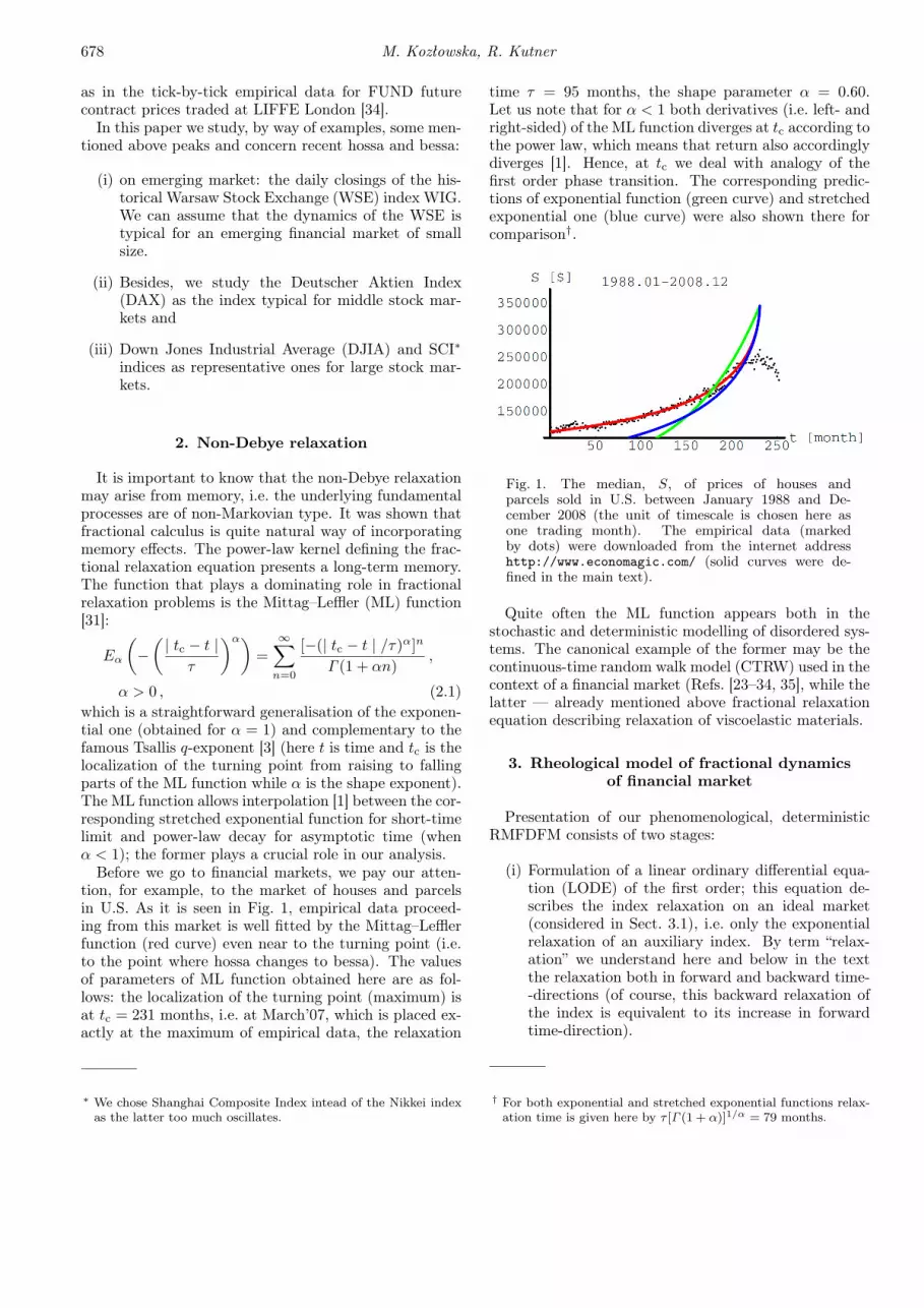
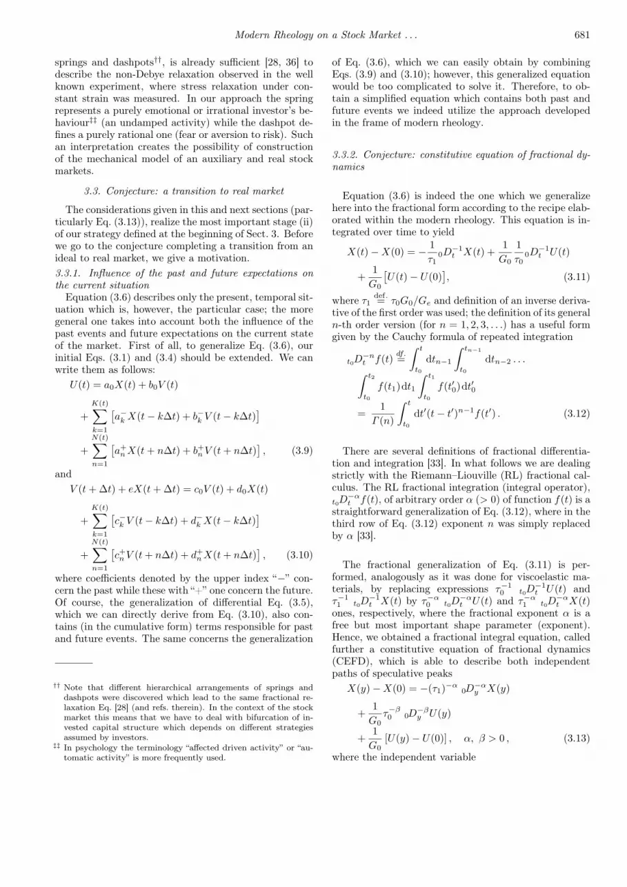
As a simple test of validity of our rheological model offractional dynamics of financial market, one can fit theformula (3.16), where we set ∆ω = 0, to empirical dataforming recent hossa of index WIG (cf. Fig. 2). It is seenthat the fit (depicted by the red curve and consideredas a trend) is satisfactory and the distribution of empiri-cal points around the trend seems to have the statisticalcharacter. However, parameters τ1 and X1 are burdenedwith huge dispersions.

This case (observed within our deterministic approach)seems to be a typical one for any hossa. It suggests theexistence of a financial uncertainty principle (FUP) ofquantities substantial to reach a profit by any investor§§.

§§ Uncertainty, together with risk and profit, were thoroughly and

Modern Rheology on a Stock Market . . . 683

This principle can be formulated as follows: among quan-tities whose values have to be known to reach a profit dur-ing the hossa, at least one is unmeasurable, i.e. its valuecannot be determined with sufficient precision. Other-wise, the profit could be obtained without any risk which

would be in contradiction to the market paradigm sayingthat market eliminates the arbitrage opportunity. For-tunately, due to anticorrelations existing between thesequantities, the summarized dispersion can be sufficientlysmall to make the total fit satisfactory.

widespreadly reviewed in book [43].

TABLE II

Fit parameters describing recent peaks of typical main indices of small, middle andlarge stock markets (upper elements L and R labeling parameters, designate left andright paths of a peak, respectively).

Parameter WIG DAX DJIA SCItLc 892± 73 969± 1 627± 3 350± 2

tRc 810± 0 940± 0 640± 0 282± 0

τL1 105± 420 426± 391 333± 38 196± 15

τR1 272± 20 426± 72 165± 191 138± 8

αL 0.57± 0.23 0.52± 0.03 1.29± 0.02 1.39± 0.02

αR 1.562± 0.025 1.12± 0.03 1.938± 0.575 1.30± 0.13

ωL 0.004± 0.001 0.004± 0 0.011± 0.0 0.075± 0.001

ωR 0.043± 0.001 0.009± 0.0 0.030± 0.070 0.051± 0.001

∆ωL 0.0± 0.0 0.0± 0.0 0.022± 0.0 0.0± 0.0

∆ωR 0.007± 0.0 0.025± 0.0 0.040± 0.070 0.0± 0.0

TABLE III

Calibrating fit parameters describing peaks of the same indices as shown in Table II.

Parameter [p] WIG DAX DJIA SCIXL

0 + XL1 60081± 85273 4698± 82 3486± 40 4810± 75

XR0 + XR

1 41963± 334 5464± 70 4010± 110 3846± 39

XL1 −8659± 2352 −763± 35 −332± 28 −217± 13

XR1 −2528± 269 −847± 36 −866± 81 153± 16

Moreover, we found that in the case of index WIGthe shape exponent αL is smaller than 1 (having a rea-sonable small dispersion, cf. the corresponding numbershown in Table II at the cross of the second column andsixth row). Hence, the fitted (solid red) curve accelerateswhen it moves toward tc, where its derivative diverges. Itsuggests that we have to deal at this singular point withthe analog of the first order phase transition on the War-saw Stock Exchange. Thus we can identify at least a partof the crash phase region as the one placed in the vicinityof the singularity, where (to good approximation) bothcurves (red and blue shown in Fig. 2) coincide. Withinthis region small change of time causes large change ofindex, which can be one of the sources of a huge disper-sion of some parameters. Below, we extended this discus-sion by considering recent daily peaks of indices listed in

Sect. 1. Full peaks of indices WIG, DAX, DJIA and SCIwere presented in subsequent Figs. 3–6 while correspond-ing fit parameters were shown in Tables II–IV (so far, inTable V important dates were presented concerning tc’sshown in Table II). Again, satisfactory agreement withempirical data are observed, which even makes possibleto draw some general conclusions.

It is seen from Table II that:

• the range of the hossa shape exponent α is largerthan 0 and smaller than 2 for considered peaks.Moreover, for large stock markets (such as NewYork Stock Exchange (NYSE) and Shanghai ones)they are even larger than 1. For bessa shape expo-nents they are all larger than 1. All these observa-tions seem to be true also for other recent peaks of

684 M. Kozłowska, R. Kutner

Fig. 2. Recent hossa of index WIG (the daily clos-ing value measured in conventional points) dated from2004.02.06 (or 2749 stock market session) to 2007.07.06and consisting of 860 sessions. The empirical data aremarked by black dots, the prediction of formula (3.16)for ∆ω = 0 is given by red solid curve while blue solidcurve is prediction of the stretched exponential functionplotted for the same parameters (shown in Tables IIand III) except parameter X1 that was set to zero. Thetime tmax denotes the position of the empirical hossa’smaximum and tc — the location of the theoretical turn-ing point (from hossa to bessa) common for both func-tions.

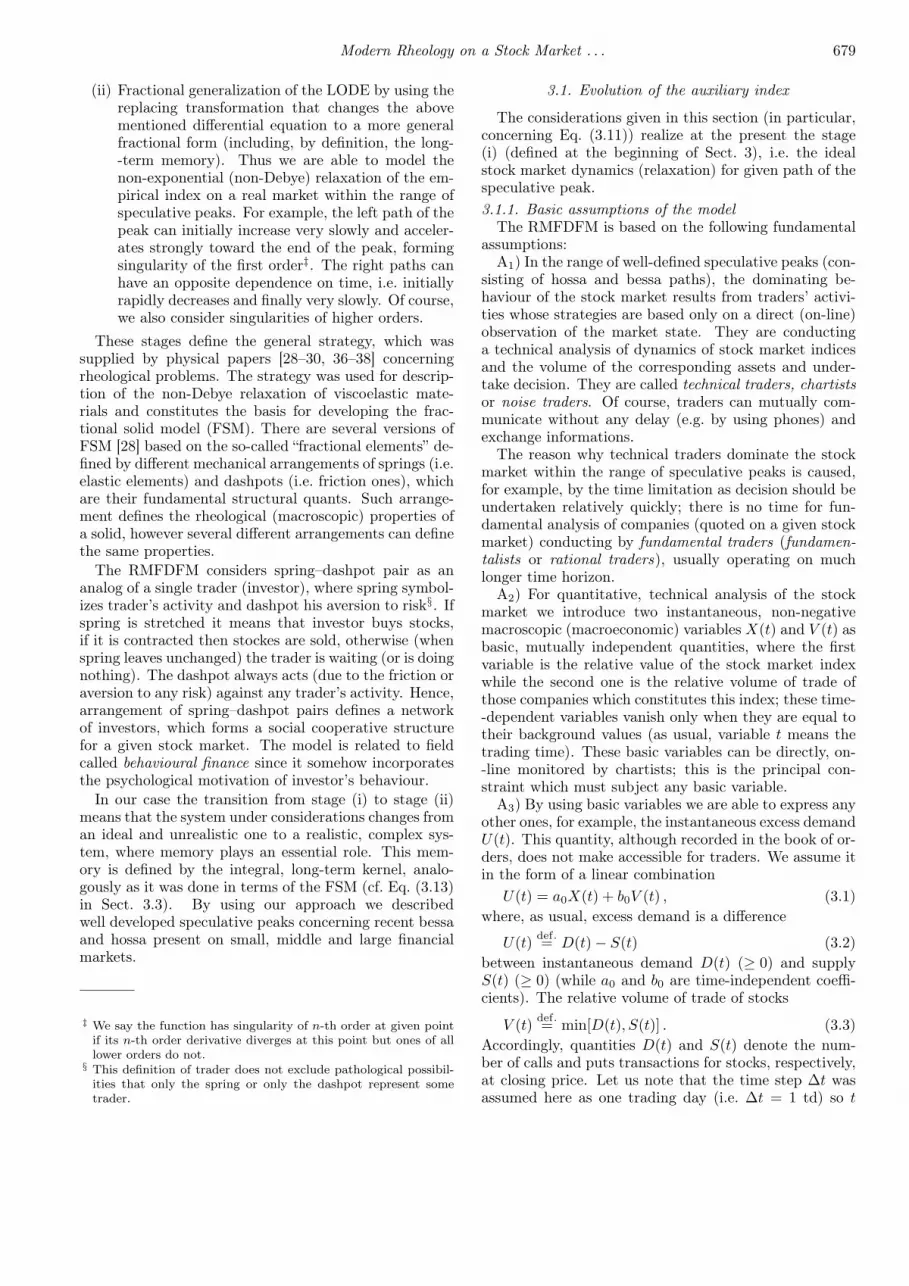
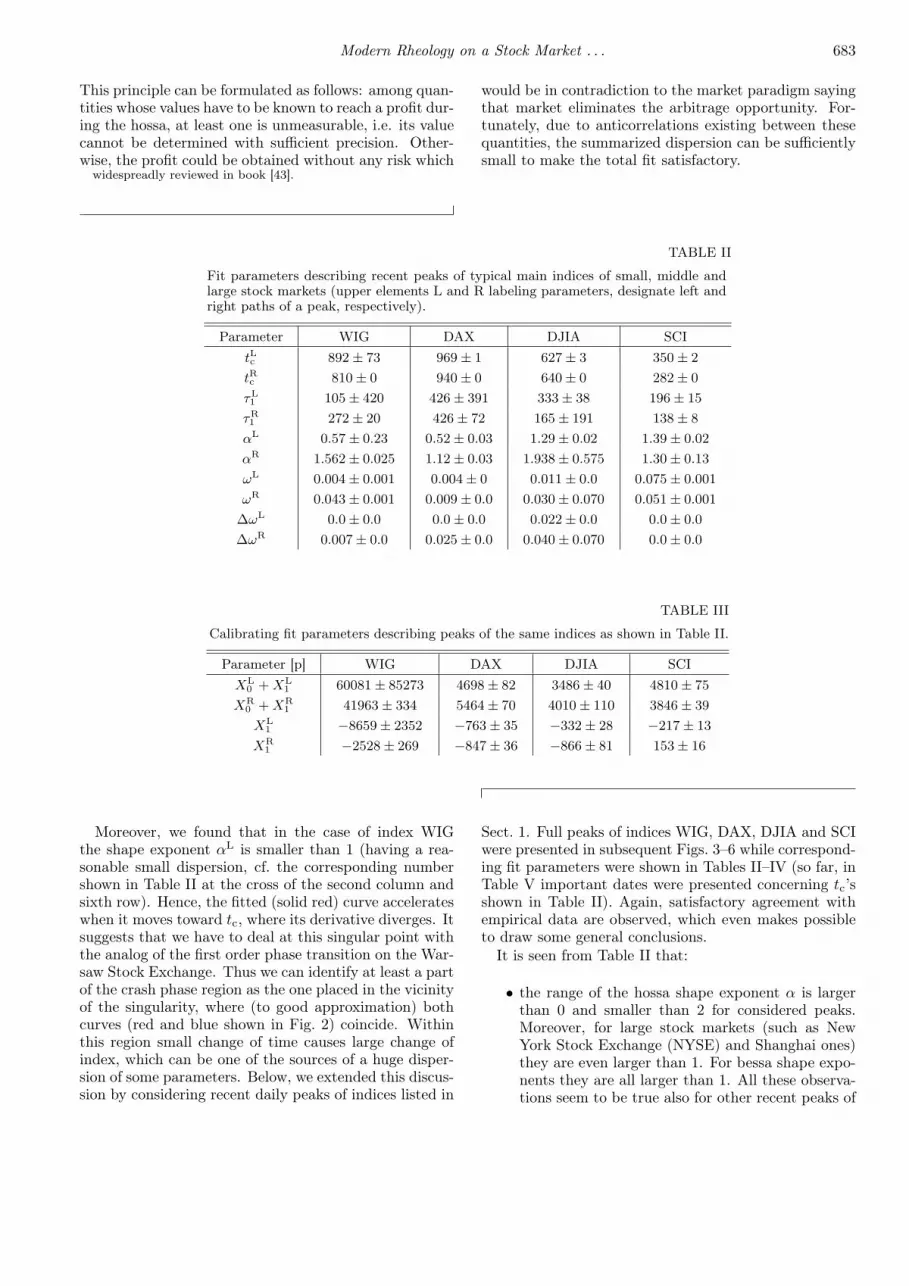
Fig. 3. Recent (full) peak of WIG extending from2004-02-06 (or from the 2750th stock market session)to 2009-05-18 (or to the 4073rd session). A little over-lap between the (theoretical) rising and falling paths atthe top of the peak is seen. This is caused by the uncer-tainty concerning the theoretical beginning of the bessaand the assumption that both paths can be consideredas independent ones. Here, the theoretical beginningof the bessa was assumed as 2007-04-24 (or the 3559thstock market session).

TABLE IVAccuracy of the fit, where fit parameters were shownin Tables II and III.

Fit accuracy WIG DAX DJIA SCIR2

L 0.9986 0.9985 0.9996 0.9983R2

R 0.9985 0.9977 0.9971 0.9967

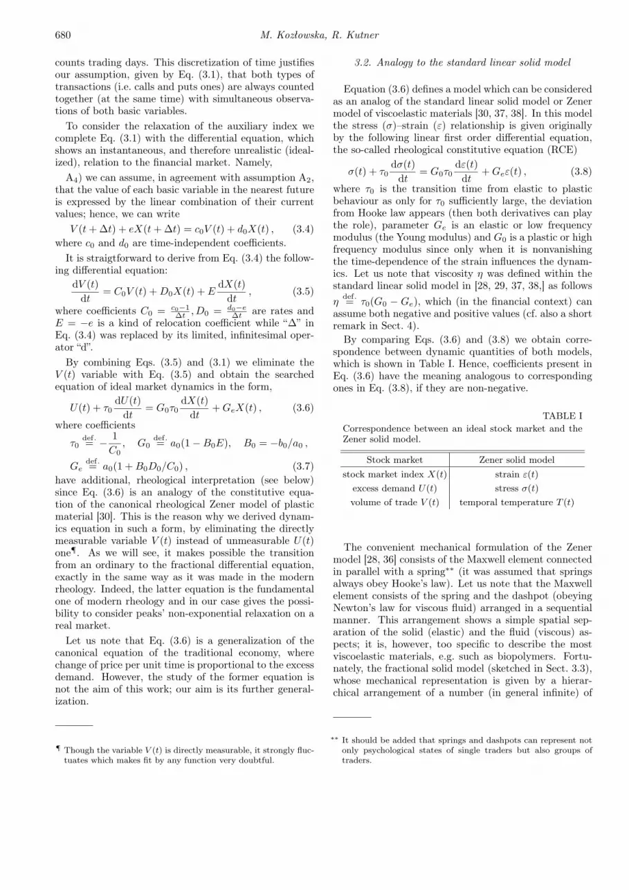
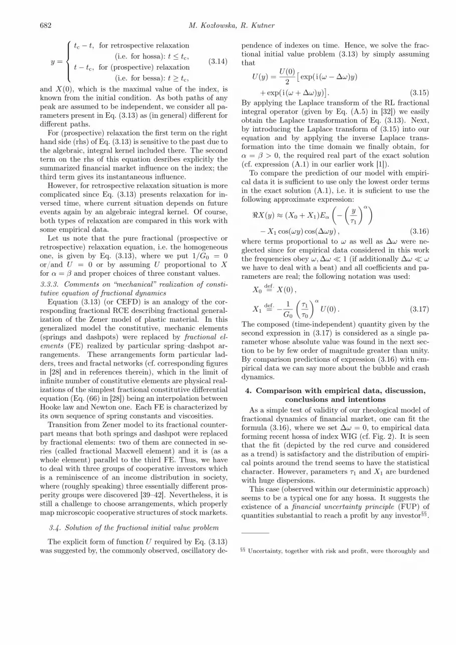
Fig. 4. Recent (full) peak of DAX extending from2003-09-04 (or from the 11001st stock market session)to 2009-07-01 (or to the 12482nd session). The (theo-retical) left path of the peak ends at 2007-07-13 (or endsat the 11985th session) while the right one begins from2007-07-12 (or begins from the 11984th session). A lit-tle discontinuity of paths and their slight displacement isseen at the top of the peak. Again, this results from theuncertainty concerning the theoretical beginning of thebessa and treating of both paths as independent ones.

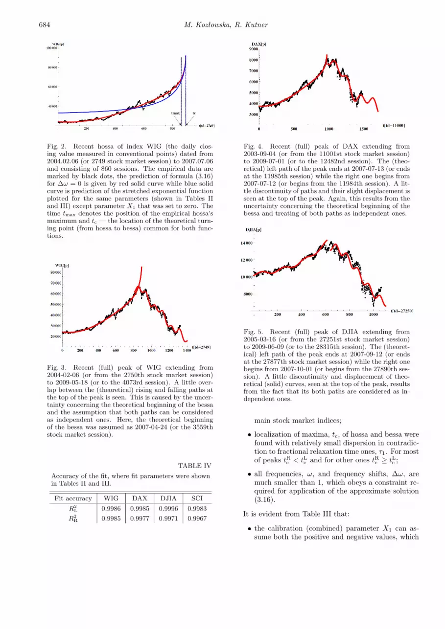
Fig. 5. Recent (full) peak of DJIA extending from2005-03-16 (or from the 27251st stock market session)to 2009-06-09 (or to the 28315th session). The (theoret-ical) left path of the peak ends at 2007-09-12 (or endsat the 27877th stock market session) while the right onebegins from 2007-10-01 (or begins from the 27890th ses-sion). A little discontinuity and displacement of theo-retical (solid) curves, seen at the top of the peak, resultsfrom the fact that its both paths are considered as in-dependent ones.

main stock market indices;

• localization of maxima, tc, of hossa and bessa werefound with relatively small dispersion in contradic-tion to fractional relaxation time ones, τ1. For mostof peaks tRc < tLc and for other ones tRc ≥ tLc ;

• all frequencies, ω, and frequency shifts, ∆ω, aremuch smaller than 1, which obeys a constraint re-quired for application of the approximate solution(3.16).

It is evident from Table III that:

• the calibration (combined) parameter X1 can as-sume both the positive and negative values, which

Modern Rheology on a Stock Market . . . 685

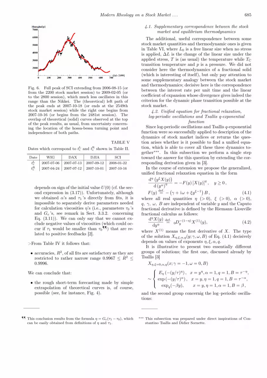
Fig. 6. Full peak of SCI extending from 2006-08-15 (orfrom the 2200 stock market session) to 2009-02-05 (orto the 2800 session), which much less oscillates in thisrange than the Nikkei. The (theoretical) left path ofthe peak ends at 2007-10-18 (or ends at the 2549thstock market session) while the right one begins from2007-10-16 (or begins from the 2481st session). Theoverlap of theoretical (solid) curves observed at the topof the peak results, as usual, from uncertainty concern-ing the location of the hossa-bessa turning point andindependence of both paths.

TABLE VDates which correspond to tLc and tRc shown in Table II.

Date WIG DAX DJIA SCItLc 2007-07-06 2007-07-13 2007-09-12 2008-01-22tRc 2007-04-24 2007-07-12 2007-10-01 2007-10-16

depends on sign of the initial value U(0) (cf. the sec-ond expression in (3.17)). Unfortunately, althoughwe obtained α’s and τ1 ’s directly from fits, it isimpossible to separately derive parameters neededfor calculation viscosities η’s (i.e., parameters τ0 ’sand Ge ’s, see remark in Sect. 3.3.2. concerningEq. (3.11)). We can only say that we cannot ex-clude negative values of viscosities (which could oc-cur if τ1 would be smaller than τ0

¶¶) that are re-lated to positive feedbacks [2].

>From Table IV it follows that:

• accuracies, R2, of all fits are satisfactory as they arerestricted to rather narrow range 0.9967 ≤ R2 ≤0.9996.

We can conclude that:

• the rough short-term forecasting made by simpleextrapolation of theoretical curves is, of course,possible (see, for instance, Fig. 4).

¶¶ This conclusion results from the formula η = Ge(τ1 − τ0), whichcan be easily obtained from definitions of η and τ1.

4.1. Supplementary correspondence between the stockmarket and equilibrium thermodynamics

The additional, useful correspondence between somestock market quantities and thermodynamic ones is givenin Table VI, where L0 is a free linear size when no stressis applied, ∆L is the change of the linear size under theapplied stress, T is (as usual) the temperature while TC

transition temperature and p is a pressure. We did notconsider here the thermodynamics of a fractional solid(which is interesting of itself), but only pay attention tosome supplementary analogy between the stock marketand thermodynamics; decisive here is the correspondencebetween the interest rate per unit time and the linearcoefficient of expansion whose divergence gives indeed thecriterion for the dynamic phase transition possible at thestock market.

4.2. Unified equation for fractional relaxation,log-periodic oscillations and Tsallis q-exponential

functionSince log-periodic oscillations and Tsallis q-exponential

function were so successfully applied to description of thedynamics of stock market indices or returns the ques-tion arises whether is it possible to find a unified equa-tion, which is able to cover all these three dynamics to-gether∗∗∗. In this subsection we perform a single steptoward the answer for this question by extending the cor-responding derivation given in [3].

In the course of extension we propose the generalized,unified fractional relaxation equation in the form

dη(yξX(y)

)

d (yα)η = −F (y) [X(y)]q , y ≥ 0 ,

F (y) def.= − (γ + iω + ξyξ−1

)B , (4.1)

where all real quantities η (> 0), ξ (> 0), α (> 0),q, γ, ω, B are independent of variable y and the Caputofractional derivative is defined by the Riemann–Liouvillefractional calculus as follows:

dηX(y)dyη

def.= 0D−(1−η)y X(1)(y), (4.2)

where X(1) means the first derivative of X. The typeof the solution Xη,ξ,α,q(y; γ, ω, B) of Eq. (4.1) decisivelydepends on values of exponents η, ξ, α, q.

It is illustrative to present two essentially differentgroups of solutions; the first one, discussed already byTsallis [3]

Xη,ξ=0,α,q(x; γ = −1, ω = 0, B)

∼

Eη (−(y/τ)η) , x = yη, α = 1, q = 1, B = τ−η,

exp (−(y/τ)α) , x = y, η = 1, q = 1, B = τ−α,

expq(−βy), x = y, η = 1, α = 1, B = β ,

and the second group concernig the log–periodic oscilla-tions:

∗∗∗ This subsection was prepared under direct inspirations of Con-stantino Tsallis and Didier Sornette.

686 M. Kozłowska, R. Kutner

Xη=1,ξ=1,α=1,q=1(x; γ, ω,B = 1) ∼ 1− [(1− δγ,1)B1y

γ

+δγ,1B2 ln(y)][

1 + C cos (ω ln(y) + φ)]. (4.3)

Of course, to find general solution of Eq. (4.1), whichseems to be a challenge, some initial or/and boundaryconditions are required.

Finally, we suppose the rheological model of fractionaldynamics of financial market, together with above men-tioned fits by log–periodic oscillations and q-exponential

function, can rationally decrease the risk of investmenton a stock market since it allows to warn the investorsbefore the stock market reaches a crash region. We hopethat our approach will be an inspiration for futher appli-cations, generalizations and study of not only the dynam-ics but also microscopic cooperative structures of stockmarkets.

TABLE VICorrespondence between some stock market and thermodynamic quantities.

Stock market Thermodynamicsstock market index X linear size L (= L0 + ∆L)

y = t− tc y = T − TC

returns per unit time d ln Xdy

linear coefficient of expansion ( ∂ ln L∂T

)p

Acknowledgments

The authors are very grateful to Didier Sornette andConstantino Tsallis for their valuable comments and sug-gestions. This work was partially supported by PolishGrant No. 119 obtained within the First Competition ofthe Committee of Scientific Research organized by Na-tional Bank of Poland.

AppendixExact solution of the fractional initial value

problem

The real part of the exact solution of our fractionalinitial value problem (3.13) takes, for α = β, the followingform:

<X(y) = (X0 + X1)Eα

(−

(y

τ1

)α)

−X1 cos(ωy) cos(∆ωy)

−ωX1

(1−

(τ0

τ1

)α) ∫ y

0

sin(ω(y − y′))

× cos(∆ω(y − y′))Eα

(−

(y′

τ1

)α)dy′

−∆ωX1

(1−

(τ0

τ1

)α) ∫ y

0

cos(ω(y − y′))

× sin(∆ω(y − y′))Eα

(−

(y′

τ1

)α)dy′. (A.1)

In all our calculations we used approximate solution givenby the first and second rows in (A.1), i.e. we assumedthat both ω and ∆ω are at most of the order of 0.1 (cf.Table II) and the fraction ( τ0

τ1)α at most of the order

of 1, which makes our fit consistent (in spite of that, wehave empirical data insufficient to verify the value of thisfraction).

References

[1] M. Kozłowska, A. Kasprzak, R. Kutner, Int. J. Mod.Phys. C 19, 453 (2008).

[2] D. Sornette, Why Stock Markets Crash. CriticalEvents in Complex Financial Systems, Princeton Uni-versity Press, Princeton 2003.

[3] C. Tsallis, Braz. J. Phys. 39, 337 (2009).[4] B.M. Roehner, Patterns of Speculation. A Study

in Observational Econophysics, Cambridge UniversityPress, Cambridge UK 2002.

[5] M. Ausloos, in: Econophysics and Sociophysics.Trends and Perspectives, Eds. B.K. Chakrabarti,A. Chakraborti, A. Chatterjee, Wiley-VCH Verlag,Weinheim 2006, Ch. 9, p. 249.

[6] W.-X. Zhou, D. Sornette, Physica A 330, 543 (2003).[7] W.-X. Zhou, D. Sornette, Physica A 330, 584 (2003).[8] P. Gnaciński, D. Makowiec, Physica A 344, 322

(2004).[9] S. Drożdż, F. Grummer, F. Ruf, J. Speth, Physica A

324, 174 (2003).[10] S. Drożdż, J. Kwapień, P. Oświecimka, J. Speth, Acta

Phys. Pol. A 114, 539 (2008).[11] D. Sornette, A. Johansen, J.-P. Bouchaud, J. Phys. I

France 6, 167 (1996).[12] D. Sornette, A. Johansen, Physica A 245, 411 (1997).[13] D. Sornette, A. Johansen, Quant. Finance 1, 452

(2001).[14] A. Johansen, D. Sornette, J. Risk 4, 69 (2001).

Modern Rheology on a Stock Market . . . 687

[15] A. Johansen, Comment on Are financial crashespredictble? by L. Laloux, M. Potters, R. Cont,J.-P. Aguilar, J.-P. Bouchaud, Europhysics Lett. 60(5), 809 (2002).

[16] D. Grech, Z. Mazur, Acta Phys. Pol. B 36, 2403(2005).

[17] R. Badii, A. Politi, Complexity. Hierarchical Struc-tures and Scaling in Physics, Cambridge UniversityPress, Cambridge UK 1997.

[18] W. Paul, J. Baschnagel, Stochastic Processes. FromPhysics to Finance, Springer-Verlag, Berlin 1999.

[19] R.N. Mantegna, H.E. Stanley, An Introduction toEconophysics: Correlations and Complexity in Fi-nance, Cambridge University Press, Cambridge UK2000.

[20] J.-P. Bouchaud, M. Potters, Theory of FinancialRisks. From Statistical Physics to Risk Management,Cambridge University Press, Cambridge UK 2001.

[21] K. Ilinski, Physics of Finance. Gauge Modelling inNon-Equilibrium Pricing, Wiley, Chichester 2001.

[22] E. Scales, R. Gorenflo, F. Mainardi, Phys. Rev. E 69,011107 (2004).

[23] L. Sabatellil, S. Keating, J. Dudley, P. Richmond,Eur. Phys. J. B 27, 273 (2002).

[24] Special Issue & Directory, Nonextensive StatisticalMechanics: New Trends, New Perspectives, Euro-physicsnews 36/6 (2005).

[25] F. Schweitzer, Brownian Agents and Active Particles,Springer-Verlag, Berlin 2003.

[26] A. Bunde, J. Kantelhardt, Phys. Blätter 57, 49(2001).

[27] R. Cont, J.-P. Bouchaud, Macroecon. Dyn. 4, 170(2000).

[28] H. Schiessel, Chr. Friedrich, Blumen, in Applica-tions of Fractional Calculus in Physics, Ed. R. Hilfer,World Scientific, Singapore 2000, Chap. 7, pp. 331-376.

[29] Th.F. Nonnenmacher, R. Metzler, Applications ofFractional Calculus in Physics, Ed. R. Hilfer, WorldSci., Singapore 2000, Ch. 8, p. 377.

[30] N. Tschoegel, The Phenomenological Theory of LinearViscoelastic Behavior, Springer-Verlag, Berlin 1989.

[31] R. Richert, A. Blumen, Disorder Effects on Relax-ational Processes: Glasses, Polymers, Proteins, Eds.R. Richert, A. Blumen, Springer, Berlin 1994, Ch. 1,p. 1.

[32] R. Metzler, J. Klafter, Phys. Rep. 339, 1 (2000).

[33] P.L. Butzer, U. Westphal, Applications of FractionalCalculus in Physics, Ed. R. Hilfer, World Sci., Singa-pore 2000, Ch. 1 p. 1.

[34] F. Mainardi, M. Raberto, R. Gorenflo, E. Scales,Physica A 287, 468 (2000).

[35] R. Kutner, F. Świtała, Qunatitative Finance 3, 201(2003).

[36] H. Schiessel, A. Blumen, J. Phys. A: Math. Gen. 26,5057 (1995).

[37] W.G. Glöckle, Th.F. Nonnenmacher, Macromolecules24 6426 (1991).

[38] W.G. Glöckle, Th.F. Nonnenmacher, Rheol. Acta 33,337 (1994).

[39] P. Richmond, S. Hutzler, R. Coelho, P. Reptowicz, inRef. [9], Ch. 5, p. 131.

[40] S. Iyazima, K. Yamamoto, in: Practical Fruitsof Econophysics. Proceedings of the Third NikkeiEconophysics Symposium, Ed. H. Takayasu, Springer--Verlag, Berlin 2006, p. 344.

[41] K. Yamamoto, S. Miyazima, H. Yamamoto, T. Oht-suki, A. Fujihara, in Ref. [40], p. 349.

[42] M. Jagielski, R. Kutner, Acta Phys. Pol. A 118, 615(2010).

[43] E. Borgonovo, L. Peccati, in: Uncertainty and Risk,Eds. M. Abdellaoni, R.D. Luce, M.J. Machina, B. Mu-nier, Springer-Verlag, Berlin 2007, Part I, p. 41.