Page 1
Cognitive Diagnostic Discrimination 1
Running head: Cognitive Diagnostic Discrimination
Cognitive Diagnostic Attribute Level Discrimination Indices
Robert Henson, William Stout, Jeff Douglas, Xuming He and Louis Roussos
University of Illinois
Submitted For ETS Review for Publication
Correspondent:
Robert Henson604 Haines Blvd.Champaign, IL 61820
The research reported here was completed under the auspices of the ExternalDiagnostic Research Team, supported by Educational Testing Service. Theopinions and statements expressed herein are those of the authors and do notnecessarily reflect the position of ETS.
Page 2
Cognitive Diagnostic Discrimination 2
Abstract
Cognitively Diagnostic Models (CDMs) model the probability of correctly answering
an item as a function of an examinee’s attribute mastery pattern. Since estimation
of the mastery pattern involves more than a continuous measure of ability,
reliability concepts introduced by CTT and IRT do not apply. Henson and Douglas
(2004) define the CDI as a measure of an item’s overall discrimination power, which
indicates an item’s usefulness in examinee attribute pattern estimation. Because of
its relationship with correct classification rates, the CDI was shown to be
instrumental in cognitively diagnostic test assembly. This paper generalizes the
CDI to attribute level discrimination indices for an item. Three different attribute
level discrimination indices are defined and their relationship with correct
classification rates is explored using Monte Carlo simulations. It is found that there
are strong relationships between the defined attribute indices and correct
classification rates. Because of their relationship with attribute level correct
classification rates, one important potential application of these indices is test
assembly from a CDM calibrated item bank.
Page 3
Cognitive Diagnostic Discrimination 3
Cognitive Diagnostic Attribute Level Discrimination
Indices
Introduction
If the goal of a test is to accurately measure an examinee’s general ability,
indices exist that can provide an indication of how reliably a test measures that
ability. However, modern methods for skills diagnosis are interested in determining
mastery on K traits rather than assessing general ability. For instance, to correctly
respond to an item there is often a set of required steps that must be completed
successfully. If an examinee has mastered all of the attributes required for these
steps, it is likely that the item will be answered correctly.
Cognitive diagnostic models (CDMs) are used to estimate a (1 x K) vector, α,
indicating each examinee’s pattern of mastery for a set of attributes given the
dichotomously scored responses to the items in a test for a set of examinees. In
addition, an (J x K) indicator matrix, Q, where J is the number of items, is used to
specify which items require what attributes. Specifically, if qjk = 1 the kth attribute
is required by the jth item and if qjk = 0 the kth attribute is not required by the jth
item.
An example of a cognitive diagnostic model, which will be used throughout
this paper as an example1, is the Reparameterized Unified Model (DiBello, Stout,
and Roussos, 1995, Hartz, 2002). Other examples of cognitively diagnostic models
exist and include the DINA (Junker and Sijtsma, 2001), NIDA (Maris, 1999), and
several others. The Reparameterized Unified Model, RUM, includes three different
Page 4
Cognitive Diagnostic Discrimination 4
item parameters, π∗j , r∗jk, and Pcj, for j = 1, . . . , J (number of items) and
k = 1, . . . , K (number of attributes). The probability of a correct response for the
ith examinee given α and ηi is:
P (Xij = 1|αi, ηi) = π∗jK∏
k=1
r∗(1−αik)qjk
jk Pcj(ηi), (1)
Here, π∗j is the probability of correctly applying all required attributes for the jth
item given the examinee has mastered all required attributes for that item, r∗jk
represents the discrimination of the jth item for the kth attribute (notice r∗ is a I x
K matrix), qjk is an indicator for whether the jth item requires mastery of the kth
attribute, Pcjis the Rasch Model with difficulty parameter −cj, and ηi is a general
measure of the ith examinee’s knowledge not otherwise specified by the Q-matrix. In
the current research cj is assumed to equal ∞ and therefore Pcj= 1 and is excluded
from the model.
As was mentioned, CDMs model the probability of correctly answering an
item as a function of an examinee’s attribute mastery pattern. Since estimation of
the mastery pattern involves more than estimation of a continuous ability, measures
of reliability initially introduced by CTT and IRT do not apply. For example, the
concept of reliability in CTT is defined as the proportion of the variance of the
observed score that can be accounted for by the variance of the continuous latent
true score (Lord & Novick, 1968). However, in CDMs, an individual is or is not
correctly classified and therefore the interpretation of a reliability coefficient such as
Cronbach’s α is not the same as the interpretation when using CTT. Also, the
concept of Fisher information is no longer applicable. Mathematically, Fisher
information is defined as the negative expectation of the second derivative of the
log-likelihood for a specified ability (Lord, 1980). Since attribute patterns are in a
Page 5
Cognitive Diagnostic Discrimination 5
discrete space, it is not possible to compute the Fisher information at a specific
attribute pattern. In summary, there is not a clear choice of index that measures
the effectiveness of a skills diagnostic test such as CTT’s reliability or IRT’s Fisher
information.
Instead of the indices, or measures, that are traditionally used in CTT or IRT,
Henson and Douglas (2004) suggest using the the CDI as a measure of an item’s
(or test’s) discrimination power. The CDI is a Kullback-Leibler based index that is
related to the distances between the item response probability distributions for each
attribute pattern. They show that the CDI strongly relates to the average correct
classification rates of examinees for a test. Because of this, Henson and Douglas
(2004) show that the CDI can be a useful index for item selection in test assembly.
Specifically, to assemble a test from an item bank, those items with the largest
CDIs should be selected first. Given the relationship between the CDI and average
correct classification rates across attributes, this test will have a high correct
classification rate when compared to all other tests that could be constructed from
the same item bank.
Because the CDI is a summary of the item’s overall discriminating power, it
does not indicate an item’s discrimination power for a specific attribute. In
addition, by its definition, the CDI ignores which attributes are required by which
items (that is Q). If items are selected based only on the CDI, it would be possible
to construct a test who’s items measure one or more of the test’s attributes poorly.
Therefore, it is necessary to expand the CDI to a set of indices that measure the
discrimination power of an item for each attribute, which incorporates Q. If the
attribute level indices are constructed similar to the CDI, one would expect an
Page 6
Cognitive Diagnostic Discrimination 6
attribute discrimination index to have a strong association with correct
classification rates for that attribute. Those tests, with only items where attribute
indices are large will also have high correct classification rates. In addition, item
selection for test assembly based on attribute discrimination indices will not suffer
from the same limitations as the CDI. In particular, constructing tests that satisfy
correct classification rates requirements for each attribute should be possible,
solving an important test assembly problem.
We propose three attribute discrimination indices. Because the discrimination
indices are based on the Kullback-Leibler information, as is the CDI, we provide a
description of the Kullback-Leibler information. Then, the three attribute
discrimination indices are discussed and a Monte Carlo simulation study is used to
demonstrate the strong relationship between each index and correct classification
rates.
Kullback-Leibler Information
Kullback-Leibler information, (Lehmann & Casella, 1998), is generally thought
of as a measure of distance between any two probability distributions, f(x) and
g(x). The Kullback-Leibler information (about the distribution f) is defined as
K[f, g] = Ef
[log
[f(X)
g(X)
]], (2)
where the measure K[f, g] is equal to the expectation, assuming f(x) is the true
distribution, of the log-likelihood ratio of any two probability density functions f(x)
and g(x). X denotes the random data and can be a scalar or vector. K[f, g] is
similar to a distance measure in that as it increases it is easier to statistically
discriminate between the two distributions (Lehmann & Casella, p. 259). In
Page 7
Cognitive Diagnostic Discrimination 7
addition K[f, g] ≥ 0, with equality when and only when f equals g.
Kullback-Leibler information is not new to educational assessment. Chang and
Ying (1996) suggest using the Kullback-Leibler information instead of Fisher
information as a more effective index for item selection in computer adaptive tests
based on IRT models. The Kullback-Leibler information in IRT can be thought of
as global information where Fisher information is local. More specifically, Fisher
information describes the ability to differentiate among abilities that are close to
one another. Specialized to the unidimensional IRT setting, Kullback-Leibler
information is defined for all ability pairs θ and θ′ (Chang, & Ying, 1996). Unlike
Fisher information, Kullback-Leibler information does not require that the
parameter space is a continuum and is hence suitable for CDMs where the attribute
vector, α, is a discrete parameter. Therefore, it is our intent to generalize Chang’s
and Ying’s (1996) results using Kullback-Leibler information as a basis for skills
diagnostic test construction with CDMs.
As in IRT, for the CDMs considered here the item response, X, is a
dichotomous variable (i.e., an examinee either gets the item right or wrong.) In
addition, the probability distribution of X, Pα(X), depends on the pattern of
attribute mastery, α, and therefore the results from Chang and Ying (1996) easily
generalize to CDMs. According to Kullback-Leibler information, an item is useful in
determining the difference between the true attribute mastery pattern, α, and an
alternative attribute mastery pattern, α′, if Kullback-Leibler information for the
comparison of Pα(X) and Pα′(X),
K[α, α′] = Eα
[log
[Pα(X)
Pα′(X)
]], (3)
is large, where Pα(X) and Pα′(X) are the probability distributions of X
Page 8
Cognitive Diagnostic Discrimination 8
conditional on α and α′, respectively.
Since X is dichotomous, (3) can be written as
1∑
x=0
Pα(x)log[
Pα(x)
Pα′(x)
],
namely
Pα(1)log[
Pα(1)
Pα′(1)
]+ Pα(0)log
[Pα(0)
Pα′(0)
].
Pα(1) and Pα′(1) are defined as the probability of a correct response using the
Reparameterized Unified Model (RUM), and Pα(0) = 1− Pα(1).
It is also possible to compute attribute pattern based Kullback-Leibler
information at the test level. Kullback-Leibler information for a test compares the
probability distribution for a test vector of J item responses, X, given attribute
pattern, α, when compared to the probability distribution of X given an alternative
attribute pattern, α′. The Kullback-Leibler test information can be written as
Kt[α,α′] = Eα
[log
[Pα(X)
Pα′(X)
]]. (4)
Since one assumption of latent cognitive diagnostic models is independence among
items conditional on the attribute patterns α2, (4) can be written as
Kt[α,α′] = Eα
[J∑
j=1
log[
Pα(Xj)
Pα′(Xj)
]],
which simplifies to
Kt[α, α′] =J∑
j=1
Eα
[log
[Pα(Xj)
Pα′(Xj)
]]. (5)
Equation 5 is the sum of the Kullback-Leibler information for each item in the
exam. Thus, the Kullback-Leibler test information is additive over items, an
important and useful property. Kt[α,α′] has an interpretation related to the power
Page 9
Cognitive Diagnostic Discrimination 9
of the likelihood ratio test for the null hypothesis that the true parameter is α
versus the alternative hypothesis that the true parameter is α′, conducted at a fixed
significance level (Rao, 1962). To be specific, if βJ(α, α′) denotes the probability of
a type II error for a test of length J , the following relationship holds,
limJ→∞
log[βJ(α, α′)]−KtJ [α, α′]
= 1.
Thus, the Kullback-Leibler information for discriminating between α and α′ is (for
a long test) monotonically related to the power of the most powerful test (the
likelihood ratio test) of α versus α′.
One complication of Kullback-Leibler information is that it only compares two
attribute patterns when there are 2K possible attribute mastery patterns. Since
Kullback-Leibler information is not symmetric, there are a total of 2K(2K − 1)
possible comparisons. To organize the 2K(2K − 1) comparisons of all attribute
pattern pairs for the jth item, it is natural to define a (2K x 2K) matrix, KLj, such
that each u, v element (u, v indexing possible attribute patterns) equals
KLjuv = Eαu
[log
[Pαu(xj)
Pαv(xj)
]].
For example, if the RUM is used
KLjuv = π∗jK∏
k=1
r∗(1−αuk)qjk
jk log[π∗j
∏Kk=1 r
∗(1−αuk)qjk
jk
π∗j∏K
k=1 r∗(1−αvk)qjk
jk
]
+ (1− π∗jK∏
k=1
r∗(1−αuk)qjk
jk )log[1− π∗j
∏Kk=1 r
∗(1−αuk)qjk
jk
1− π∗j∏K
k=1 r∗(1−αvk)qjk
jk
](6)
where, it is assumed for simplicity that all cj = ∞ and αuk represents the kth
element of the attribute mastery vector, αu. Notice that if one has an item bank of
N items, KLj can be computed for each item j. The elements of each KLj that are
Page 10
Cognitive Diagnostic Discrimination 10
large indicate the attribute pattern pairs that the jth item is most useful in
discriminating among. In addition, the total Kullback-Leibler information matrix
can be defined for any test of J items, KLt, by simply summing across the KLj of
the items selected. To construct a test one might, for example, choose items such
that all of the elements in KLt are large and therefore the power to discriminate
between any two attribute patterns is high.
Discrimination
Theoretically, each element of KLt could function as an indicator of how well
α is measured when compared to α′. However, in applications, it is not reasonable
to simultaneously consider the 2K(2K − 1) discrimination indices of an exam.
Therefore to produce a useful indication of test discrimination, it is imperative that
a single index, such as the CDI or 2K attribute level indices of discrimination,
based on the entries of KLt, be defined. Specifically, the kth discrimination index
should be useful to predict the correct classification rate achieved by an effective
statistical procedure for the kth attribute for a given test.
It should be noted that, while correct classification of an attribute has been
discussed generically (i.e., correct classification of an attribute), there are two
important components to correct classification, the correct classification rate of the
masters, p(αk = 1|αk = 1), and the correct classification rate of the nonmasters,
p(αk = 0|αk = 0). The purpose of the test (e.g., including differing costs and
differing benefits of correct classification) can often times determine whether the
correct classification of masters, or the correct classification of nonmasters, is more
important. Therefore, instead of only defining a single discrimination index for the
Page 11
Cognitive Diagnostic Discrimination 11
kth attribute, a discrimination index will be defined to help predict the correct
classification rate of the masters for the kth attribute, δk(1), and a discrimination
index to help predict the correct classification rate of nonmasters, δk(0).
It is our intent to show that effective indices at the attribute level can be
computed from the Kullback-Leibler matrix, KLt. In addition, by using only linear
combinations of the elements of KLt, the defined attribute discrimination index for
a test is simply the sum of each corresponding item attribute discrimination index
(that is additivity holds across items), which will allow attribute specific test
construction in a similar manner as described by Henson and Douglas (2004). The
following subsections provide definitions of three promising indices of attribute
discrimination, each with their benefits and limitations.
Attribute Discrimination Index A (δAk )
Recall that some elements within KL are more important than others. Notice
that by using the attribute patterns that only differ on the kth attribute, the
corresponding KLjuv’s describe the extent to which a master can be discriminated
from a nonmaster, or a nonmaster from a master, on the kth attribute while holding
attribute mastery constant on the remaining (K − 1) attributes.
Of the attribute comparisons that differ only by the kth attribute, there are
2(K−1) comparisons describing the discrimination power of masters from nonmasters
on the kth attribute (i.e., comparing attribute patterns such that αk = 1 and
α′k = 0), and there are 2(K−1) comparisons describing the discrimination power of
nonmasters from masters on the kth attribute (i.e, attribute patterns such that
αk = 0 and α′k = 1). The first index will compute the mean of the elements in KLj
that satisfy the constraints just defined previously. Specifically, equations (7) and
Page 12
Cognitive Diagnostic Discrimination 12
(8) provide formal definitions of δAk (1) and δA
k (0) in terms of the comparisons made
in KL.
δAjk(1) =
1
2(K−1)
∑
Ω1
KLj(α,α′) (7)
δAjk(0) =
1
2(K−1)
∑
Ω0
KLj(α,α′) (8)
where
Ω1 ∈ αk = 1 ∩ α′k = 0 ∩ αv = α′v∀v 6= k (9)
and
Ω0 ∈ αk = 0 ∩ α′k = 1 ∩ αv = α′v∀v 6= k. (10)
Index δAjk provides a simple measure of the average discrimination that an item
contains about attribute k while controlling for the remaining attributes. It does
not incorporate prior knowledge about the testing population and therefore assumes
that all attribute patterns are equally likely. If the jth item does not measure the
kth attribute (i.e., the j, k element of the Q-matrix is 0) then that item contains no
information about attribute mastery for the kth attribute and therefore δAjk(1) and
δAjk(0) are zero. While the index has been defined at the item level, the test
discrimination, δAk , is the sum across each item discrimination as given in (11).
δAtk =
J∑
j=1
δAjk (11)
The additivity of item discrimination is because the elements in KLj are additive as
described previously.
Page 13
Cognitive Diagnostic Discrimination 13
Attribute Discrimination Index B (δBk )
Though there are times when an individual may not have prior knowledge of
the specific population, often prior testing has been used to calibrate the items and
therefore there is some knowledge of the population characteristics. For example,
Hartz (2002) estimates attribute associations and the population probability of
mastery using the Fusion Model to fit the RUM. If the Fusion Model is fitted, prior
probabilities of attribute patterns are estimated. In addition, it can be argued that,
in general, there are not many cases such that all attribute patterns are equally
likely. Therefore, a second index, δBjk, is defined, as in equations (12) and (13), such
that the expectation given the distribution of α is used (i.e., the prior probabilities,
or estimates of the prior probabilities, of the attribute patterns are used to weight
the appropriate elements of KLj).
δBjk(1) = Eα[KLj(α,α′)|Ω1] (12)
δBjk(0) = Eα[KLj(α,α′)|Ω0] (13)
where Ω1 and Ω0 are defined in (9) and (10), respectively.
Provided that the distribution of α is known, or can be estimated, equation
(12) can be rewritten as,
δBk (1) =
∑
Ω1
wKL(α, α′), (14)
where
w = P (α|αk = 1),
and (13) can be rewritten as,
δBk (0) =
∑
Ω0
wKL(α, α′), (15)
Page 14
Cognitive Diagnostic Discrimination 14
where
w = P (α|αk = 0).
Like δAjk, δB
jk provides a simple measure of discrimination but prior population
information is used to weight the elements of KLj giving those values for which α is
more likely higher weights than less likely attribute patterns. δBjk is interpreted as
the amount of information, about attribute k, provided by an item. It should be
noticed that, if all P (α|αk = 1) are equal, then δBjk(1) = δA
jk(1) and, if all
P (α|αk = 0) are equal, then δBjk(0) = δA
jk(0). Therefore δAjk is a special case of δB
jk.
Again, as in the discrimination index, δAjk, additivity holds:
δBtk =
J∑
j=1
δBjk. (16)
Attribute Discrimination Index C (δCk )
Both δAjk and δB
jk are useful indices for discrimination in that they measure the
discriminating power of an item in assessing the kth attribute. However, the intent
is to define an index that is most strongly associated with correct classification
rates. It is possible that δAk and δB
k are not taking full advantage of all the
information available. As an illustrative example, if two attributes k and k′ are
perfectly correlated (i.e., if an examinee is a master of attribute k then he or she is
also a master of attribute k′, and if an examinee is a nonmaster of attribute k then
he or she is also a nonmaster of attribute k′), then by knowing attribute k is
mastered by an examinee and the fact that the correlation between k and k′ is 1,
attribute k′ is also known to be mastered by the examinee. Therefore, an item that
contains information about attribute k can also provide information about k′, even
if the item does not require k′ for its solution. A discrimination index may need to
Page 15
Cognitive Diagnostic Discrimination 15
incorporate all the information provided from the association between attributes, if
such information is available.
The index δCjk assumes that if attributes are associated, the discrimination of
the kth attribute provided by an item is a function of both the information about αk
contained in the item and the information provided from the known or estimated
associations of αk with other attributes measured by the test. Abstractly speaking,
to incorporate the additional information provided from the association of other
attributes, associated attributes are first re-expressed as a function of a set of newly
defined independent attributes. The likelihood functions used to compute entries of
a KLj can then be re-expressed as a function of the independent attributes and the
Kullback-Leibler information computed for all attribute pairs. Notice that since the
true attributes are associated, each attribute will typically be a function of more
than one of the independent attributes. For this reason, it is possible for an item
that does not measure αk to provide information about αk.
Specifically, we define a set of independent attributes for the ith subject,
α∗1, · · · , α∗K , such that P (α∗k′ = 1|α∗k∀k 6= k′) = P (α∗k′ = 1) for all k 6= k′. To compute
the discrimination index for the kth attribute, the association of each attribute with
the kth attribute is modeled by expressing the true attributes for the ith examinee,
αi1, · · · , αiK , as a function of the independent attributes as given in (17),
αim = bimα∗ik + (1− bim)α∗im;∀i = 1, . . . , I. (17)
Here, bim is a random Bernoulli variable for the ith examinee with probability pbm
and all bim are assumed to be independent in m for each fixed i. By definition, as
the association between the attributes increases the pbm are chosen to be larger.
However, one must consider that for a randomly selected examinee all 2K sequences
Page 16
Cognitive Diagnostic Discrimination 16
of the bm’s for m = 1, . . . , K are possible (since all bm are random independent
Bernoulli variables). Bl will be used to denote the vector of the lth possible
combination of b1, · · · , bK , where l = 1, . . . , 2K.The RUM is written in terms of the independent attributes using equation
(17) and the Kullback-Leibler matrix with respect to attribute k, KLljk for the jth
item and lth combination of (b1, · · · , bK), denoted Bl = (Bl1, · · · , Bl
K), can be
computed. It should be noted that in the Kullback-Leibler equation (6), all of the
attributes α∗1, . . . , α∗K now potentially play a role, as determined by Bl via Equation
(17). In addition, for any KLljk, discrimination indices for the kth attribute, ∆l
jk(1)
and ∆ljk(0), can be computed using the equations analogous to δB
k (1) and δBk (0)
written in terms of the independent attributes, α∗1, . . . , α∗K . Specifically,
∆ljk(1) =
∑
α∗∈Ω∗1k
wKLljk(α
∗,α′∗), (18)
where
w = P (α∗|elements in Ω∗1k),
and
∆ljk(0) =
∑
α∗∈Ω∗0k
wKLljk(α
∗,α′∗), (19)
where
w = P (α∗|elements in Ω∗0k).
Here Ω∗1k and Ω∗
0k are defined as
Ω∗1k = α∗k = 1 ∩ α′k
∗= 0 ∩ α∗v = α′v
∗∀v 6= k (20)
and
Ω∗0k = α∗k = 0 ∩ α′k
∗= 1 ∩ α∗v = α′v
∗∀v 6= k. (21)
Page 17
Cognitive Diagnostic Discrimination 17
Notice that KLljk is computed for all 2K vectors Bl. In addition, ∆l
jk(1) and
∆ljk(0) can be computed for each KLl
jk. We define the discrimination indices δCjk(1)
and δCjk(0) as the expectation of ∆l
jk(1) and ∆ljk(0), respectively, across all possible
combinations Bl for all l = 1, . . . , 2K, as determined by the Bernoulli trials
distribution for Bl.
δCjk(1) = EBl
[∆ljk(1)] (22)
δCjk(0) = EBl
[∆ljk(0)] (23)
Equations (22) and (23) can be written as
2K∑
l=1
wl∆ljk(1) (24)
and2K∑
l=1
wl∆ljk(0) (25)
where
wl =K∏
m=1
[pBl
mbm
(1− pbm))1−Blm ]. (26)
As in the previous discrimination index, δBk , this discrimination index
incorporates information about the population by using prior probabilities of all
attribute patterns as weights to determine comparisons that are more likely. In
addition to using the prior probabilities of each attribute pattern to determine
weights, δCk also uses the association between each attribute pattern pair in defining
the individual Kullback-Leibler elements. By incorporating the association between
attributes, the discrimination of the kth attribute is a function of both the
information contained about attribute k in the item, or test, and information
provided by the estimated correlations of the other attributes with the kth attribute.
Also, additivity will hold as in δA and δB.
Page 18
Cognitive Diagnostic Discrimination 18
It should be noted that if the attributes are uncorrelated, pbk= 0 for all
k = 1, · · · , K and therefore δCk = δB
k . In addition, if all attributes are uncorrelated
and all conditional probabilities used to produce the weights for B are equal then it
is also true that δCk = δB
k = δAk .
Discrimination Index Discussion
The CDIt, δAk , δB
k , and δCk , are indices based on the Kullback-Leibler
information. However, there are some basic philosophical differences between the
indices that should be addressed. Specifically, the indices differ in the extent that
the characteristics of the population influence the value of the index and they differ
in their interpretation.
Both the test discrimination, CDI, and the attribute discrimination index A,
δAk , are computed from the Kullback-Leibler information matrix and the Hamming
distances between all pairs of attributes. They do not incorporate any
characteristics of the population (i.e., distribution probabilities of attribute
patterns) and therefore they must be considered only as a general index of the
amount of discrimination power a test provides to differentiate between any two
attribute patterns. Recall that both the discrimination indices for CTT and the
efficiency of a test in IRT are functions of the population characteristics. However,
when using either the CDI or δAk , there is an implicit assumption that items are
equally discriminating for all populations. There may be instances when a test is
less informative because many of the attribute comparisons for which the test is
highly discriminating are unlikely in the population.
Secondly, δBk and δC
k are influenced by the population parameters, but are
conceptually different in the extent to which such information is incorporated into
Page 19
Cognitive Diagnostic Discrimination 19
the index. Notice that δBk weights the comparisons by the prior probability of the
attribute pattern. Therefore, if an attribute pattern is unlikely in a population
those comparisons will have small weights. However, δBk only incorporates the
amount of discrimination contained by a test. If a test does not measure an
attribute, δBk , as well δA
k , will indicate that the test contains no direct discrimination
power about that attribute, which is different from δCk .
The attribute discrimination index δCk allows for information, in addition to
what is provided directly by the test, to contribute to the discriminating power of a
test. Specifically, if an association exists between the attributes, then δCk is defined
by the information provided by the test and the information provided from the
association with any additional attributes measured by the test. Therefore, δCk
should be interpreted as the total information provided about an attribute.
Examples
Now a simple one-item example calibrated using the RUM model will
illustrate the calculations of the four indices (i.e., δA1 (1), δB
1 (1) and δC1 (1)). The
single item has an r∗ equal to 0.125, a π∗ = .8, and a Q-matrix entry equal to (1 0).
Notice that the Q-matrix entry indicates that the first of only two attributes are
required to correctly answer the item.
To compute the CDI, δAk , and δB
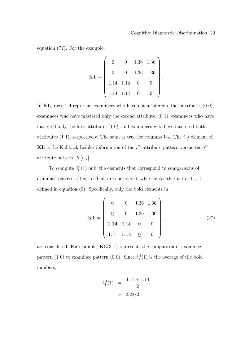
k the matrix KL must be calculated using
Page 20
Cognitive Diagnostic Discrimination 20
equation (??). For the example,
KL =
0 0 1.36 1.36
0 0 1.36 1.36
1.14 1.14 0 0
1.14 1.14 0 0
.
In KL, rows 1-4 represent examinees who have not mastered either attribute, (0 0),
examinees who have mastered only the second attribute, (0 1), examinees who have
mastered only the first attribute, (1 0), and examinees who have mastered both
attributes (1 1), respectively. The same is true for columns 1-4. The i, j element of
KL is the Kullback-Leibler information of the ith attribute pattern versus the jth
attribute pattern, K[i, j].
To compute δA1 (1) only the elements that correspond to comparisons of
examinee patterns (1 x) to (0 x) are considered, where x is either a 1 or 0, as
defined in equation (9). Specifically, only the bold elements in
KL =
0 0 1.36 1.36
0 0 1.36 1.36
1.14 1.14 0 0
1.14 1.14 0 0
. (27)
are considered. For example, KL(3, 1) represents the comparison of examinee
pattern (1 0) to examinee pattern (0 0). Since δA1 (1) is the average of the bold
numbers,
δA1 (1) =
1.14 + 1.14
2
= 2.28/2
Page 21
Cognitive Diagnostic Discrimination 21
= 1.14.
The discrimination index can also be computed for attribute 2, δA2 (1), using the
italicized values in 27. Since the item does not require attribute 2, δA2 (1) = 0. Using
similar equations δA1 (0) and δA
2 (0) can be computed.
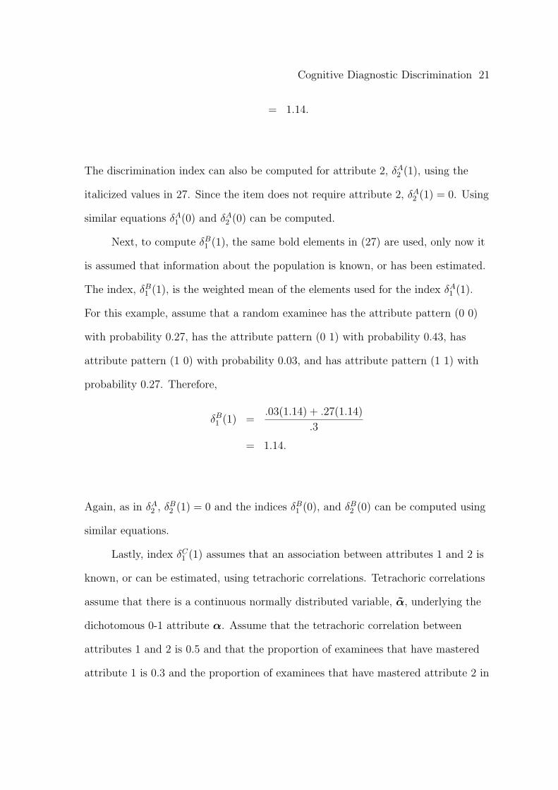
Next, to compute δB1 (1), the same bold elements in (27) are used, only now it
is assumed that information about the population is known, or has been estimated.
The index, δB1 (1), is the weighted mean of the elements used for the index δA
1 (1).
For this example, assume that a random examinee has the attribute pattern (0 0)
with probability 0.27, has the attribute pattern (0 1) with probability 0.43, has
attribute pattern (1 0) with probability 0.03, and has attribute pattern (1 1) with
probability 0.27. Therefore,
δB1 (1) =
.03(1.14) + .27(1.14)
.3
= 1.14.
Again, as in δA2 , δB
2 (1) = 0 and the indices δB1 (0), and δB
2 (0) can be computed using
similar equations.
Lastly, index δC1 (1) assumes that an association between attributes 1 and 2 is
known, or can be estimated, using tetrachoric correlations. Tetrachoric correlations
assume that there is a continuous normally distributed variable, α, underlying the
dichotomous 0-1 attribute α. Assume that the tetrachoric correlation between
attributes 1 and 2 is 0.5 and that the proportion of examinees that have mastered
attribute 1 is 0.3 and the proportion of examinees that have mastered attribute 2 in
Page 22
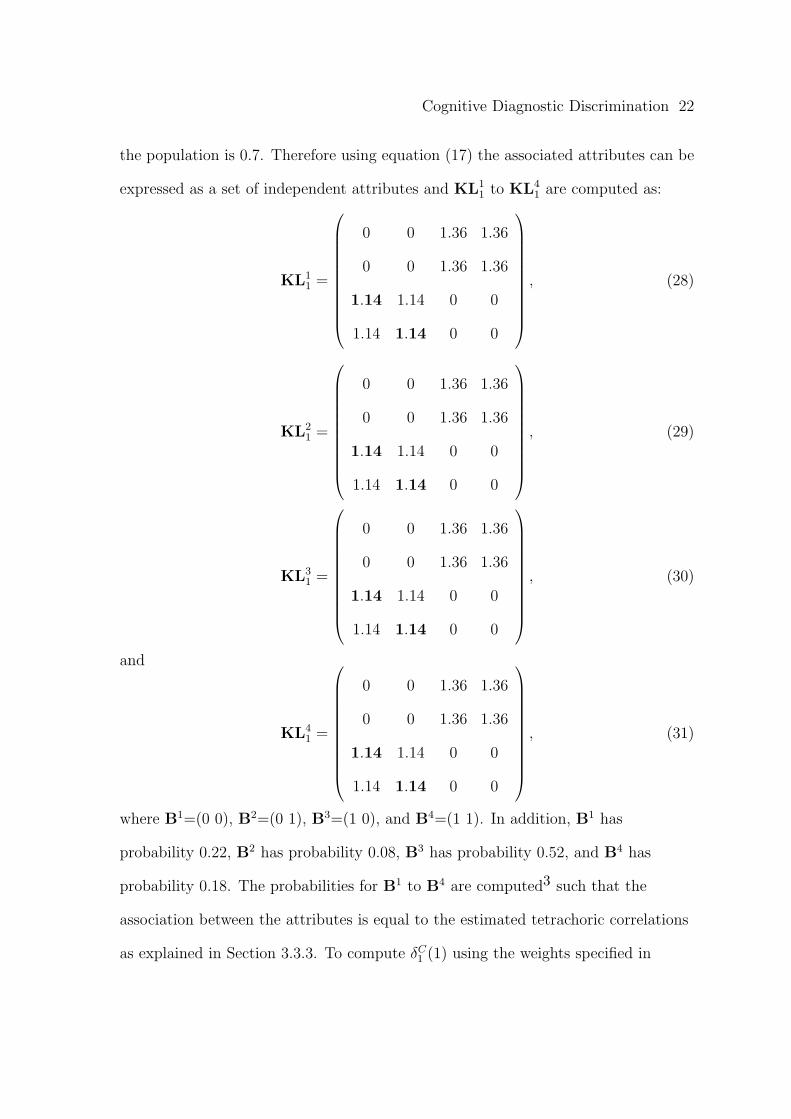
Cognitive Diagnostic Discrimination 22
the population is 0.7. Therefore using equation (17) the associated attributes can be
expressed as a set of independent attributes and KL11 to KL4
1 are computed as:
KL11 =
0 0 1.36 1.36
0 0 1.36 1.36
1.14 1.14 0 0
1.14 1.14 0 0
, (28)
KL21 =
0 0 1.36 1.36
0 0 1.36 1.36
1.14 1.14 0 0
1.14 1.14 0 0
, (29)
KL31 =
0 0 1.36 1.36
0 0 1.36 1.36
1.14 1.14 0 0
1.14 1.14 0 0
, (30)
and
KL41 =
0 0 1.36 1.36
0 0 1.36 1.36
1.14 1.14 0 0
1.14 1.14 0 0
, (31)
where B1=(0 0), B2=(0 1), B3=(1 0), and B4=(1 1). In addition, B1 has
probability 0.22, B2 has probability 0.08, B3 has probability 0.52, and B4 has
probability 0.18. The probabilities for B1 to B4 are computed3 such that the
association between the attributes is equal to the estimated tetrachoric correlations
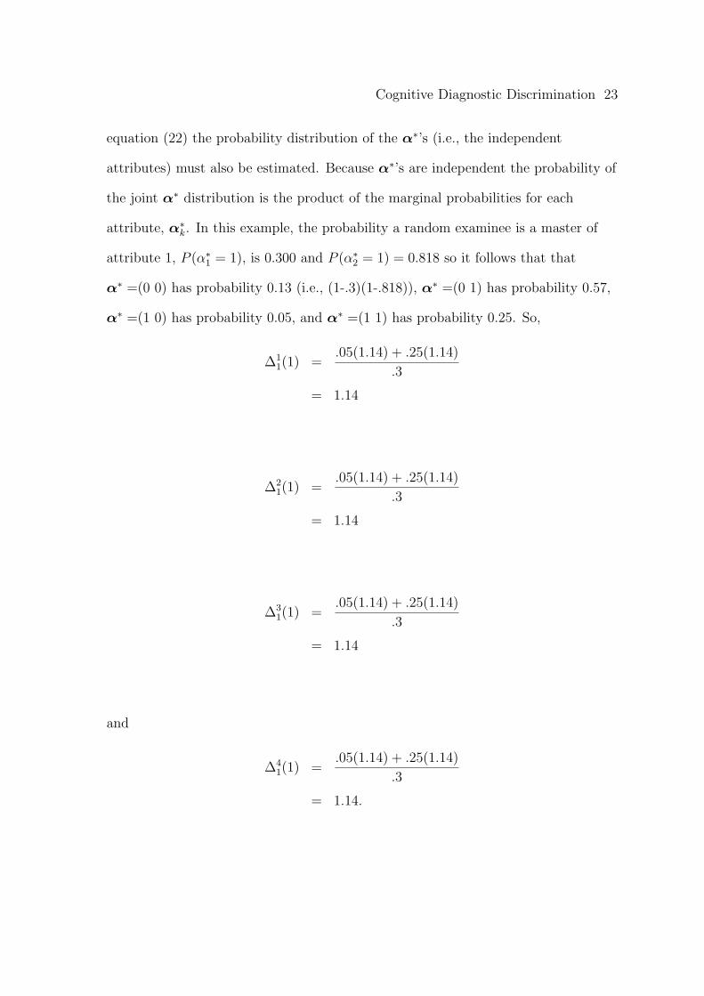
as explained in Section 3.3.3. To compute δC1 (1) using the weights specified in
Page 23
Cognitive Diagnostic Discrimination 23
equation (22) the probability distribution of the α∗’s (i.e., the independent
attributes) must also be estimated. Because α∗’s are independent the probability of
the joint α∗ distribution is the product of the marginal probabilities for each
attribute, α∗k. In this example, the probability a random examinee is a master of
attribute 1, P (α∗1 = 1), is 0.300 and P (α∗2 = 1) = 0.818 so it follows that that
α∗ =(0 0) has probability 0.13 (i.e., (1-.3)(1-.818)), α∗ =(0 1) has probability 0.57,
α∗ =(1 0) has probability 0.05, and α∗ =(1 1) has probability 0.25. So,
∆11(1) =
.05(1.14) + .25(1.14)
.3
= 1.14
∆21(1) =
.05(1.14) + .25(1.14)
.3
= 1.14
∆31(1) =
.05(1.14) + .25(1.14)
.3
= 1.14
and
∆41(1) =
.05(1.14) + .25(1.14)
.3
= 1.14.
Page 24
Cognitive Diagnostic Discrimination 24
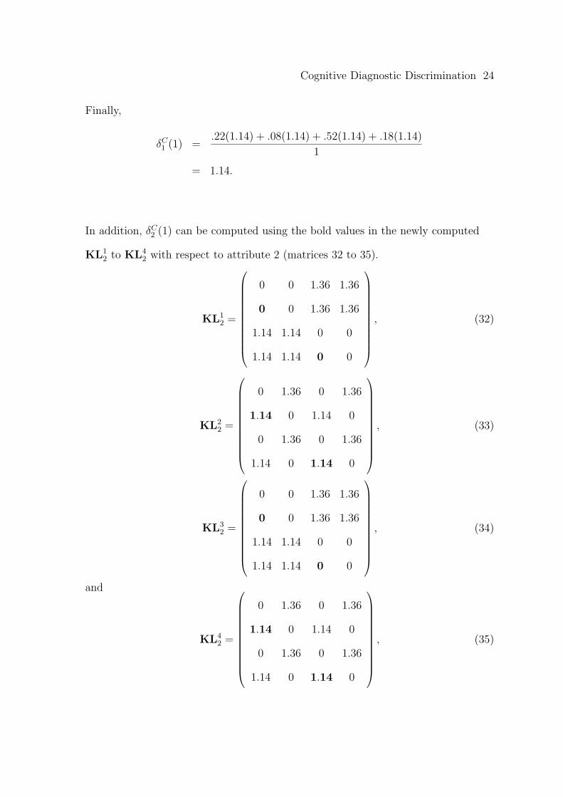
Finally,
δC1 (1) =
.22(1.14) + .08(1.14) + .52(1.14) + .18(1.14)
1
= 1.14.
In addition, δC2 (1) can be computed using the bold values in the newly computed
KL12 to KL4
2 with respect to attribute 2 (matrices 32 to 35).
KL12 =
0 0 1.36 1.36
0 0 1.36 1.36
1.14 1.14 0 0
1.14 1.14 0 0
, (32)
KL22 =
0 1.36 0 1.36
1.14 0 1.14 0
0 1.36 0 1.36
1.14 0 1.14 0
, (33)
KL32 =
0 0 1.36 1.36
0 0 1.36 1.36
1.14 1.14 0 0
1.14 1.14 0 0
, (34)
and
KL42 =
0 1.36 0 1.36
1.14 0 1.14 0
0 1.36 0 1.36
1.14 0 1.14 0
, (35)
Page 25
Cognitive Diagnostic Discrimination 25
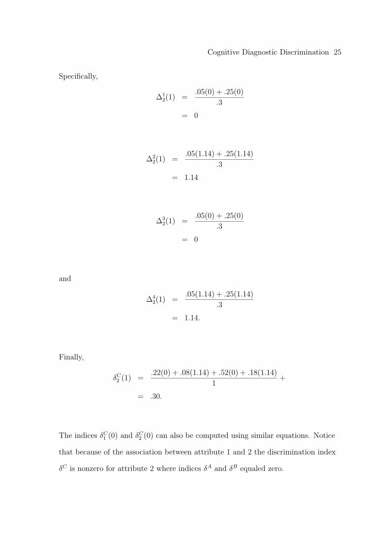
Specifically,
∆12(1) =
.05(0) + .25(0)
.3
= 0
∆22(1) =
.05(1.14) + .25(1.14)
.3
= 1.14
∆32(1) =
.05(0) + .25(0)
.3
= 0
and
∆42(1) =
.05(1.14) + .25(1.14)
.3
= 1.14.
Finally,
δC2 (1) =
.22(0) + .08(1.14) + .52(0) + .18(1.14)
1+
= .30.
The indices δC1 (0) and δC
2 (0) can also be computed using similar equations. Notice
that because of the association between attribute 1 and 2 the discrimination index
δC is nonzero for attribute 2 where indices δA and δB equaled zero.
Page 26
Cognitive Diagnostic Discrimination 26
A Simulation Study of the Performance of the Three
Indices
Using Monte Carlo simulation, random tests are generated where items are
calibrated using the RUM. For each test, δAk , δB
k , and δCk , and the responses of
10,000 simulated examinees are computed. In addition, attribute patterns of each
simulated examinee are estimated and correct classification rates for both the
masters and nonmasters are computed. Next, correlations are computed between
correct classification rates and each of the three discrimination indices in order to
assess the performance of the indices.
In the simulation study the RUM item parameters were assumed known, as
would be the case with a test bank of precalibrated items. Given a set of item
parameters comprising a test, 10,000 examinees are simulated. When generating
each set of 10,000 examinee attribute patterns it is important to consider two
aspects of the attribute pattern distribution. These are the proportion of examinees
that have mastered the kth attribute, pk, and the associations between the
attributes. In the simulation study all pk = .5 were chosen in order to control for
the influence of pk on correct classification rates. In addition, it is reasonable to
believe that the attributes are associated in the population. If an individual has
mastered one attribute, he is more likely to have mastered a second attribute
measured by the exam. Therefore, an appropriate simulation of examinees would
incorporate both specified pk’s and a specified relationship between the attributes.
A total of 10, 000 multivariate normal K-dimensional vectors
(α ∼ MV N(0,ρ)) are generated to simulate attributes that have a positive
relationship, where ρ represents a correlation matrix with equal off-diagonal
Page 27
Cognitive Diagnostic Discrimination 27
elements. Using the pk’s, a cutoff κk = 0 is computed for each attribute such that
P (α ≤ κk) = pk = .5. The ith individual’s mastery for attribute k is thus:
αik =
1 if αk ≥ 0
0 otherwise
For reasons that will become clear in the following subsections, for each test
administration a second sample, comprised of 10,000 examinees, is generated
separate from the other simulated sample of 10,000 examinees. The second sample
will be used for an accurate Monte Carlo approximation of the prior distribution of
attribute patterns, as needed for indices B and C.
Given each examinee’s attribute pattern, scores for each item are generated
based on the RUM simulated model. Given the probability of a correct response,
P (Xij = 1|α), a random U(0, 1) variable u is generated and the score Xij is:
Xij =
1 if u ≤ P (Xij = 1|α)
0 otherwise
Here, P (Xij = 1|α) is the probability of a correct response using the RUM.
Since the item parameters are known, instead of using an MCMC approach to
carry out a Baysian analysis, Baysian based classification is accomplished by
computing the likelihood for all possible attribute patterns given the examinees’
scores and multiplying by the prior probabilities of attribute patterns(estimated
from the second sample of 10,000 subjects.) The Baysian posterior mode is then
used to classify the attribute pattern for that individual. Given the estimated
attribute patterns, for each attribute the proportion of examinees for which the
attribute was correctly classified is recorded.
Next, to determine the characteristics of the simulated tests, one must
Page 28
Cognitive Diagnostic Discrimination 28
remember that the purpose of this study is to study the relationship between each
discrimination index and correct classification rates. Tests are generated that are
realistic while intentionally creating variability of the measurement quality of the
tests (i.e., some tests have high correct classification rates while others do not
perform as well). 1000 randomly generated 40-item tests are constructed to measure
5 attributes. On average, each item requires 2 attributes in each test. In addition,
item parameters are generated such that tests will range from low to high cognitive
structure. In this context, low cognitive structure will be defined as situations for
which the absence of one or more of the required attributes have a relatively small
influence on examinees’ probability of a correct item response and therefore the
items are at best moderately informative whereas in high cognitive structure the
probability of a correct response is strongly influenced by the presence or absence of
one or more of the required attributes. The characteristics of the randomly
generated item parameters for each test are as follows:
π∗’s are randomly generated from a uniform distribution, U(.85, .95) for all 1000
tests.
r∗’s are used to modify the cognitive structure. Specifically, for the ith simulation,
i = 1, . . . , 1000, r∗’s are randomly generated from a uniform distribution,
U(.1 + .6(i−1)999
, .3 + .6(i−1)999
). Notice that for the first simulation r∗’s are
generated to resemble high cognitive structure (i.e., r∗’s range from .1 to .3).
For each simulation, the range slowly shifts to resemble a lower cognitive
structure until the last simulated test contains r∗’s that range from .7 to .9,
low cognitive structure indeed.
Page 29
Cognitive Diagnostic Discrimination 29
c’s are all set to ∞ and therefore Pc(η) = 1.
It is important to remember that each index incorporates the dependence
between the attributes to a different degree. Specifically, δAk totally ignores the
association between attributes, δBk incorporates the association only in the form of
multiplicative weights (based on the prior probabilities) of the Kullback-Leibler
information, and δCk fully uses the known (or estimated in application) association
between attributes. Three different simulations of 1000 tests are run; a simulation
with all the off-diagonal elements of ρ equal to .5, a simulation with all of the
off-diagonal elements of ρ equal to .75, and a simulation with all of the off-diagonal
elements of ρ equal to .95.
Lastly, a separate simulation study is used to give an extreme example that
provides evidence for the inability of δAk and δB
k to use collateral information in the
absence of direct information about the attribute. 1000 20-item tests are generated
to measure 2 attributes such that all items only measure the second attribute and
the known correlation between attributes 1 and 2 is .999. A high correlation
between attribute 1 and attribute 2 indicates that each item that measures attribute
2 also provides information about attribute 1. That is, because of the strong
association between attributes, if attribute 2 is known, attribute 1 is known with
almost certainty. It should be noted that since none of the twenty items directly
measure attribute 1, δAk (1), δA
k (0), δBk (1) and δB
k (0) are equal to 0, where, as
appropriate, δC1 (1) ≈ δC
2 (1) and δC1 (0) ≈ δC
2 (0) can be shown. It is also true that for
attribute 2, all corresponding discrimination indices for indices A, B, and C, should
be approximately equal. The example illustrates a situation in which it is
advantageous to fully incorporate the associations between the two attributes as in
Page 30
Cognitive Diagnostic Discrimination 30
δCk . If correlations are not taken into consideration from the empirical Bayes
perspective, the test contains no direct information about attribute 1, yet there is a
large amount of information for attribute 1 provided from knowing attribute 2, so
indices δAk and δB
k are misleading.
Results
Three Simulation Studies.
For each of the basic three simulation studies, the basic descriptive statistics
of the discrimination indices and correct classification rates are provided. In
addition, the correlations between the discrimination indices and the appropriate
correct classification rates are computed. The following paragraphs first summarize
the results from the three simulations then the results from the separate simulation
study are provided.
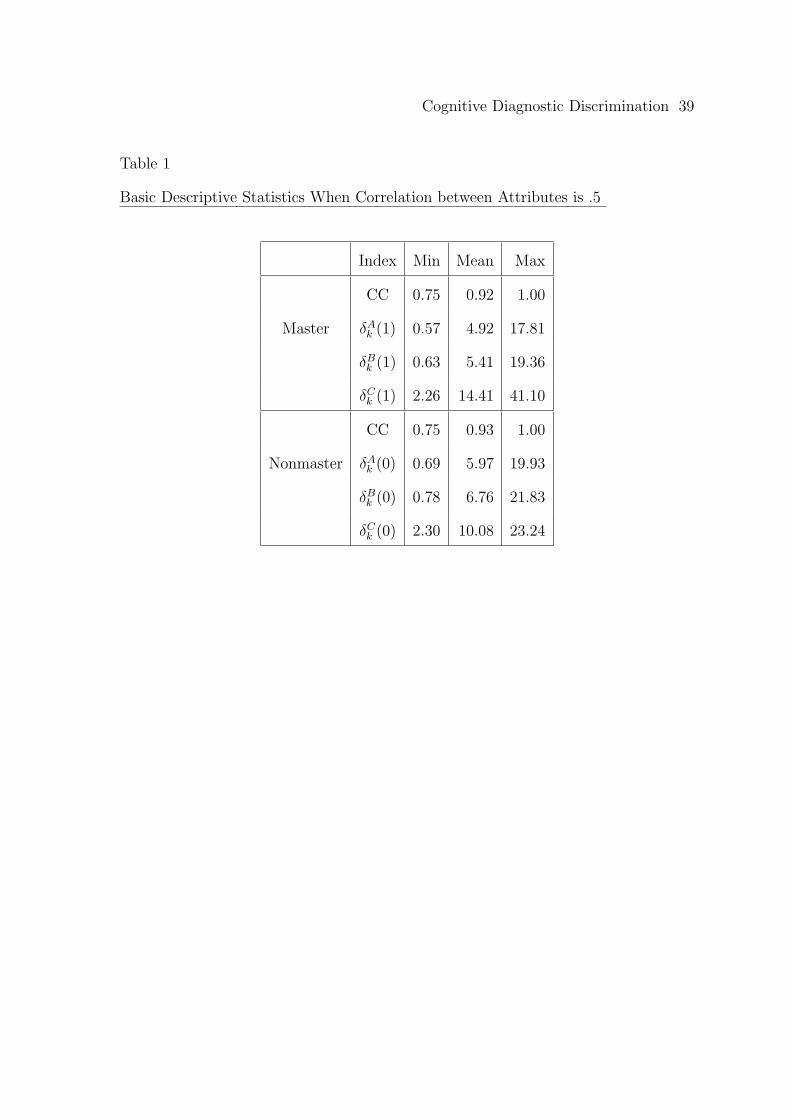
To begin, the minimum, maximum, and mean values of correct classification
rates (CC) over the 1000 simulation replications, δAk , δB
k , and of δCk , for both masters
and nonmasters, respectively, are summarized in Tables 1 to 3. It should be noted
that, since tests are randomly generated with all pk = .5 and all attribute
correlations are the same within a study, the results of the 5 attributes are
indistinguishable. Therefore, the basic descriptive statistics will be summarized
across all attributes, which provide more efficient estimates of their true values.
Insert Table 1 about here
Page 31
Cognitive Diagnostic Discrimination 31
Insert Table 2 about here
Insert Table 3 about here
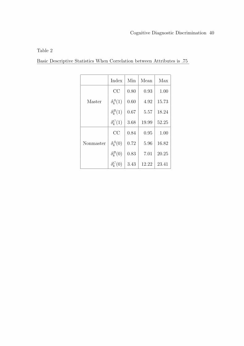
In general, while tests were developed to allow for a large range of correct
classification rates, it is clear that as the correlation between attributes increases the
range of correct classification rates are reduced. For example, the correct
classification rates for the simulation study with attributes that have correlations of
.5 range from .75 to 1.00 with an average of approximately .92, while they range
from approximately .90 to 1.00 with an average of .97 in the simulation study with
attributes that have correlations of .95. In addition, while the intent of this study is
to only define indices that correlate with correct classification rates, it can be seen
that both δAk and δB
k appear to be on similar scales where δCk , on average, is much
larger.
Next, Table 4 provides the means4 of the correlations between the correct
classification rates and δAk , δB
k , and δCk , for the masters and nonmasters. The table
shows that in general correlations are quite high and therefore it is reasonable to use
the discrimination indices as indicators of correct classification rates.
Insert Table 4 about here
Page 32
Cognitive Diagnostic Discrimination 32
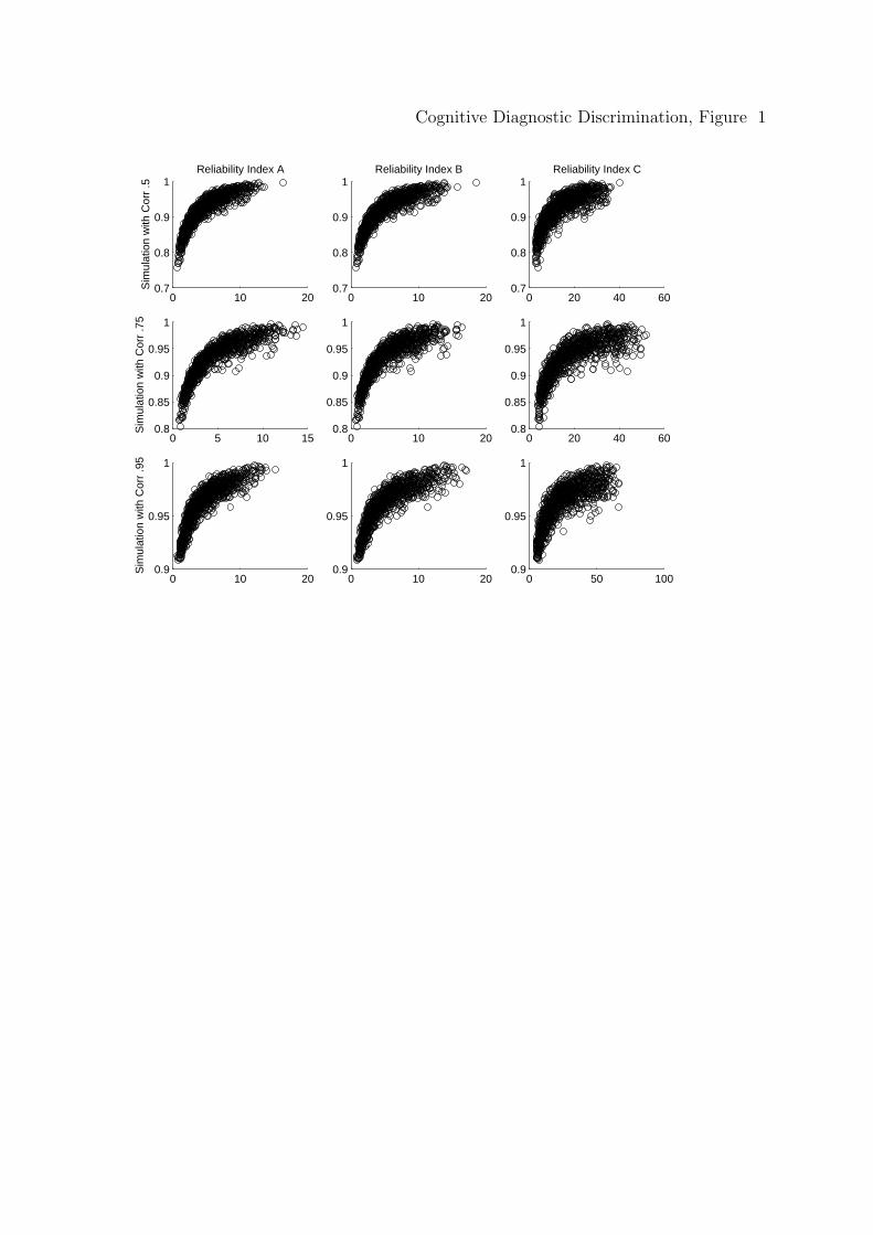
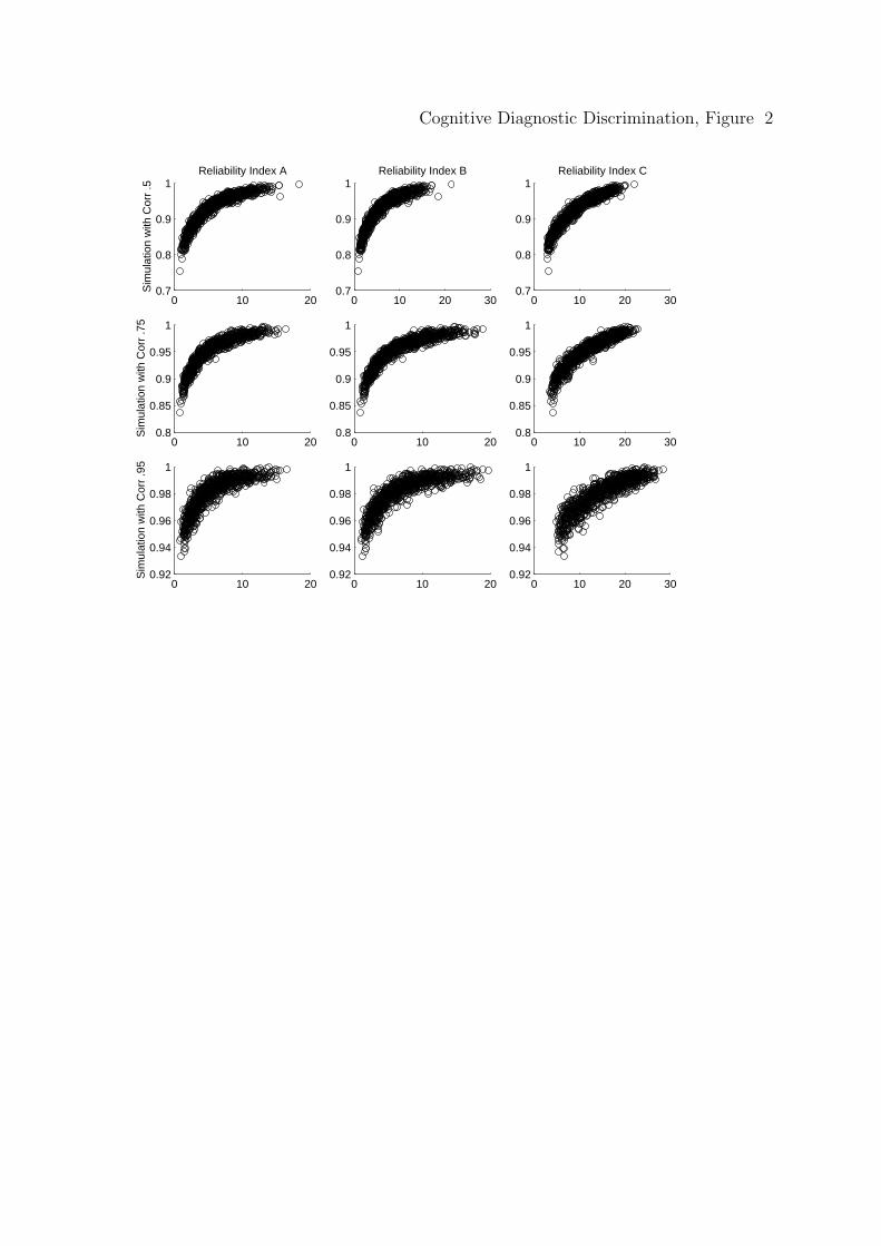
One assumption when using the correlation is that the relationship is
approximately linear. Therefore, it is important that the scatter plots be explored
for linearity. Figures 1 and 2 are scatter plots of attribute 1, as an example, for all
three indices to visually explore the relationships between discrimination and
correct classification rates for masters (Figure 1) and nonmasters (Figure 2).
Columns 1, 2, and 3 represent the plots for the discrimination indices δAk , δB
k , and
δCk , respectively, crossed with the rows, which represent the three simulations (i.e.,
when correlations between attributes are .5, .75, and .95).
Insert Figure 1 about here
Insert Figure 2 about here
Clearly the relationship is not linear due to the asymptotic effect of correct
classification rates (i.e., they approach 1). Therefore, the true relationship is
stronger than what is indicated by the correlation coefficients (i.e., if the values were
transformed such that the relationship is linear correlations will be higher). It is
also possible that some correlations are smaller due to a restricted range, which may
explain the reduction of the correlations for the simulation where all attribute have
a correlation of .95.
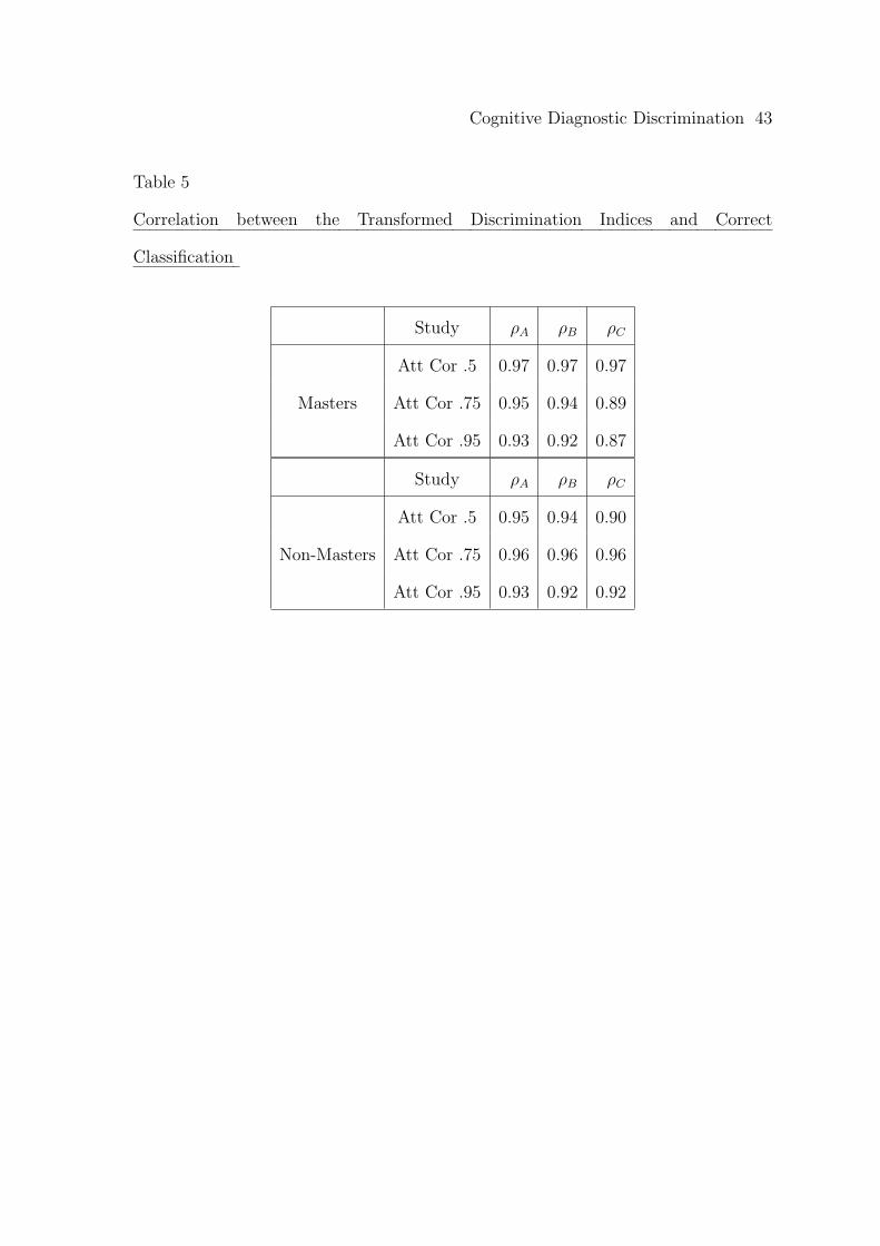
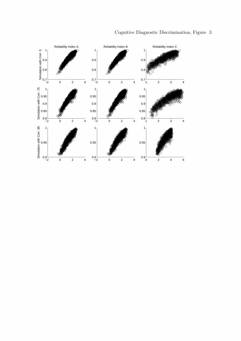
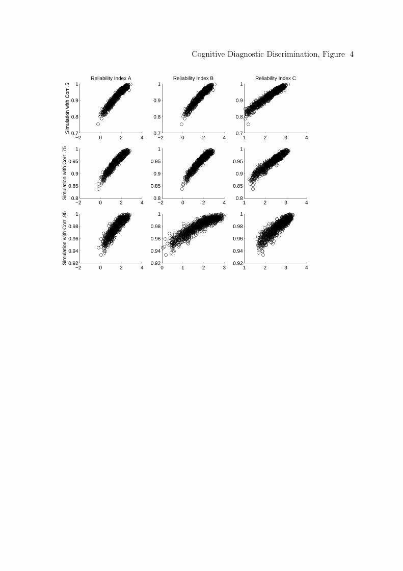
So to explore the true strength of the relationship between the discrimination,
or a monotonic function of discrimination, and correct classification, the
log-transformation of the discrimination indices can be used so that the relationship
Page 33
Cognitive Diagnostic Discrimination 33
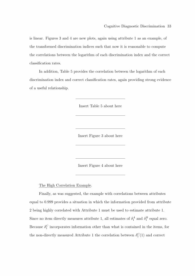
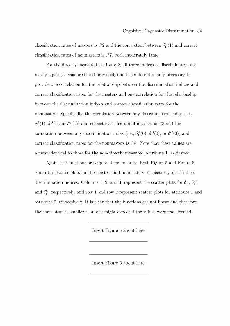
is linear. Figures 3 and 4 are new plots, again using attribute 1 as an example, of
the transformed discrimination indices such that now it is reasonable to compute
the correlations between the logarithm of each discrimination index and the correct
classification rates.
In addition, Table 5 provides the correlation between the logarithm of each
discrimination index and correct classification rates, again providing strong evidence
of a useful relationship.
Insert Table 5 about here
Insert Figure 3 about here
Insert Figure 4 about here
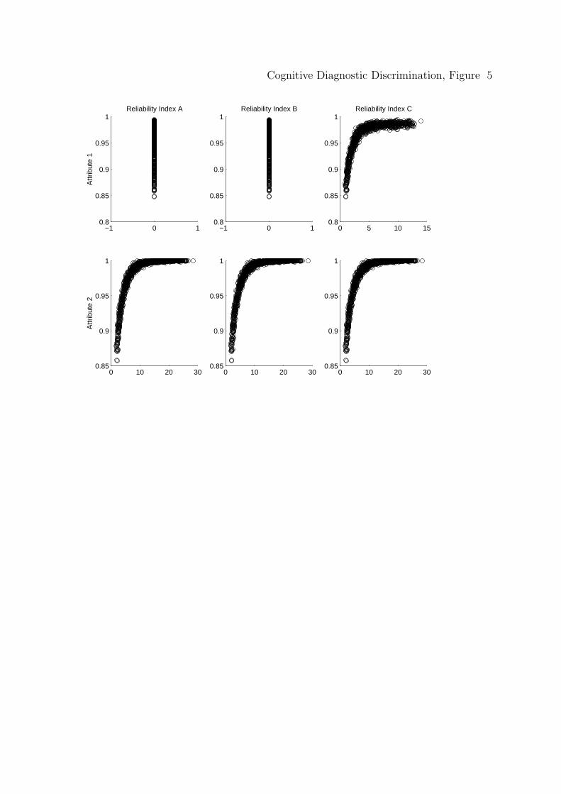
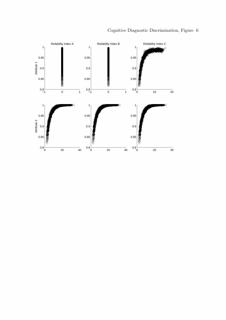
The High Correlation Example.
Finally, as was suggested, the example with correlations between attributes
equal to 0.999 provides a situation in which the information provided from attribute
2 being highly correlated with Attribute 1 must be used to estimate attribute 1.
Since no item directly measures attribute 1, all estimates of δA1 and δB
1 equal zero.
Because δC1 incorporates information other than what is contained in the items, for
the non-directly measured Attribute 1 the correlation between δC1 (1) and correct
Page 34
Cognitive Diagnostic Discrimination 34
classification rates of masters is .72 and the correlation between δC1 (1) and correct
classification rates of nonmasters is .77, both moderately large.
For the directly measured attribute 2, all three indices of discrimination are
nearly equal (as was predicted previously) and therefore it is only necessary to
provide one correlation for the relationship between the discrimination indices and
correct classification rates for the masters and one correlation for the relationship
between the discrimination indices and correct classification rates for the
nonmasters. Specifically, the correlation between any discrimination index (i.e.,
δA1 (1), δB
1 (1), or δC1 (1)) and correct classification of mastery is .73 and the
correlation between any discrimination index (i.e., δA1 (0), δB
1 (0), or δC1 (0)) and
correct classification rates for the nonmasters is .78. Note that these values are
almost identical to those for the non-directly measured Attribute 1, as desired.
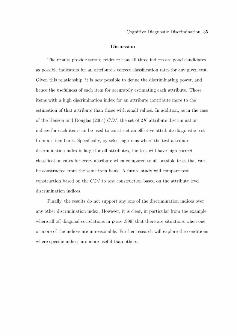
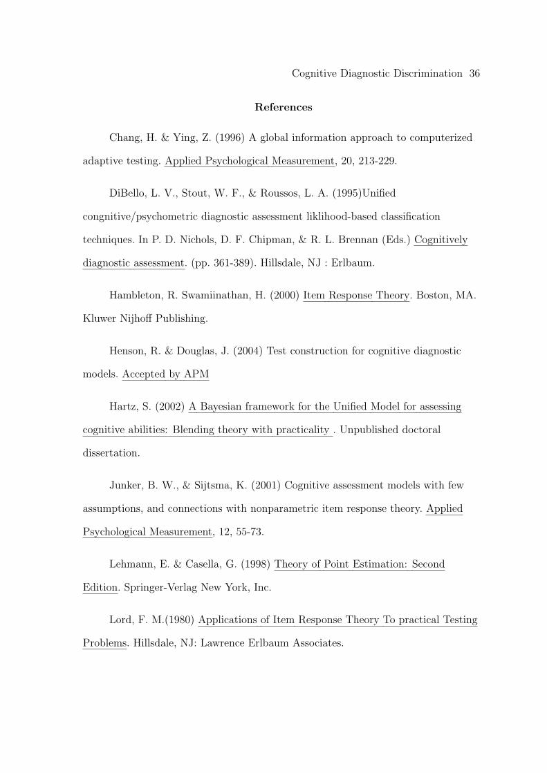
Again, the functions are explored for linearity. Both Figure 5 and Figure 6
graph the scatter plots for the masters and nonmasters, respectively, of the three
discrimination indices. Columns 1, 2, and 3, represent the scatter plots for δA1 , δB
1 ,
and δC1 , respectively, and row 1 and row 2 represent scatter plots for attribute 1 and
attribute 2, respectively. It is clear that the functions are not linear and therefore
the correlation is smaller than one might expect if the values were transformed.
Insert Figure 5 about here
Insert Figure 6 about here
Page 35
Cognitive Diagnostic Discrimination 35
Discussion
The results provide strong evidence that all three indices are good candidates
as possible indicators for an attribute’s correct classification rates for any given test.
Given this relationship, it is now possible to define the discriminating power, and
hence the usefulness of each item for accurately estimating each attribute. Those
items with a high discrimination index for an attribute contribute more to the
estimation of that attribute than those with small values. In addition, as in the case
of the Henson and Douglas (2004) CDI, the set of 2K attribute discrimination
indices for each item can be used to construct an effective attribute diagnostic test
from an item bank. Specifically, by selecting items where the test attribute
discrimination index is large for all attributes, the test will have high correct
classification rates for every attribute when compared to all possible tests that can
be constructed from the same item bank. A future study will compare test
construction based on the CDI to test construction based on the attribute level
discrimination indices.
Finally, the results do not support any one of the discrimination indices over
any other discrimination index. However, it is clear, in particular from the example
where all off diagonal correlations in ρ are .999, that there are situations when one
or more of the indices are unreasonable. Further research will explore the conditions
where specific indices are more useful than others.
Page 36
Cognitive Diagnostic Discrimination 36
References
Chang, H. & Ying, Z. (1996) A global information approach to computerized
adaptive testing. Applied Psychological Measurement, 20, 213-229.
DiBello, L. V., Stout, W. F., & Roussos, L. A. (1995)Unified
congnitive/psychometric diagnostic assessment liklihood-based classification
techniques. In P. D. Nichols, D. F. Chipman, & R. L. Brennan (Eds.) Cognitively
diagnostic assessment. (pp. 361-389). Hillsdale, NJ : Erlbaum.
Hambleton, R. Swamiinathan, H. (2000) Item Response Theory. Boston, MA.
Kluwer Nijhoff Publishing.
Henson, R. & Douglas, J. (2004) Test construction for cognitive diagnostic
models. Accepted by APM
Hartz, S. (2002) A Bayesian framework for the Unified Model for assessing
cognitive abilities: Blending theory with practicality . Unpublished doctoral
dissertation.
Junker, B. W., & Sijtsma, K. (2001) Cognitive assessment models with few
assumptions, and connections with nonparametric item response theory. Applied
Psychological Measurement, 12, 55-73.
Lehmann, E. & Casella, G. (1998) Theory of Point Estimation: Second
Edition. Springer-Verlag New York, Inc.
Lord, F. M.(1980) Applications of Item Response Theory To practical Testing
Problems. Hillsdale, NJ: Lawrence Erlbaum Associates.
Page 37
Cognitive Diagnostic Discrimination 37
Lord, F., Novick, M. (1968) Statistical Theories of mental test scores with
contributions from Alan Birnbaum. Reading, MA: Addison-Wesley.
Maris, E. (1999) Estimating multiple classification latent class models.
Psychometrika, 64, 187-212.
McDonald, R. (1999) Test Theory: A Unified treatment. Mahwah, NJ:
Lawrence Erlbaum Associates.
Rao, C. R. (1962) Efficient Estimates and optimum inference procedures in
large samples Journal of the Royal Statistics Society Series B, 24, 46-72.
Page 38
Cognitive Diagnostic Discrimination 38
Footnotes
1While the RUM is used the proposed indices apply to any cognitive diagnostic
model with a discrete latent examinee space
2It should be noted that if the RUM is used, independence is conditional on α
and η. However, if all cj’s are assumed to be ∞ (as in the computation of the three
indices presented in this paper), the test Kullback-Leibler information is equal to
the sum of the Kullback-Leibler information for all items as in (5).
3Actual computation of the probabilities involves a Monte Carlo simulation of
examinees with the specified tetrachoric correlation and proportion of masters.
4all standard errors less or equal to .01
Page 39
Cognitive Diagnostic Discrimination 39
Table 1
Basic Descriptive Statistics When Correlation between Attributes is .5
Index Min Mean Max
CC 0.75 0.92 1.00
Master δAk (1) 0.57 4.92 17.81
δBk (1) 0.63 5.41 19.36
δCk (1) 2.26 14.41 41.10
CC 0.75 0.93 1.00
Nonmaster δAk (0) 0.69 5.97 19.93
δBk (0) 0.78 6.76 21.83
δCk (0) 2.30 10.08 23.24
Page 40
Cognitive Diagnostic Discrimination 40
Table 2
Basic Descriptive Statistics When Correlation between Attributes is .75
Index Min Mean Max
CC 0.80 0.93 1.00
Master δAk (1) 0.60 4.92 15.73
δBk (1) 0.67 5.57 18.24
δCk (1) 3.68 19.99 52.25
CC 0.84 0.95 1.00
Nonmaster δAk (0) 0.72 5.96 16.82
δBk (0) 0.83 7.01 20.25
δCk (0) 3.43 12.22 23.41
Page 41
Cognitive Diagnostic Discrimination 41
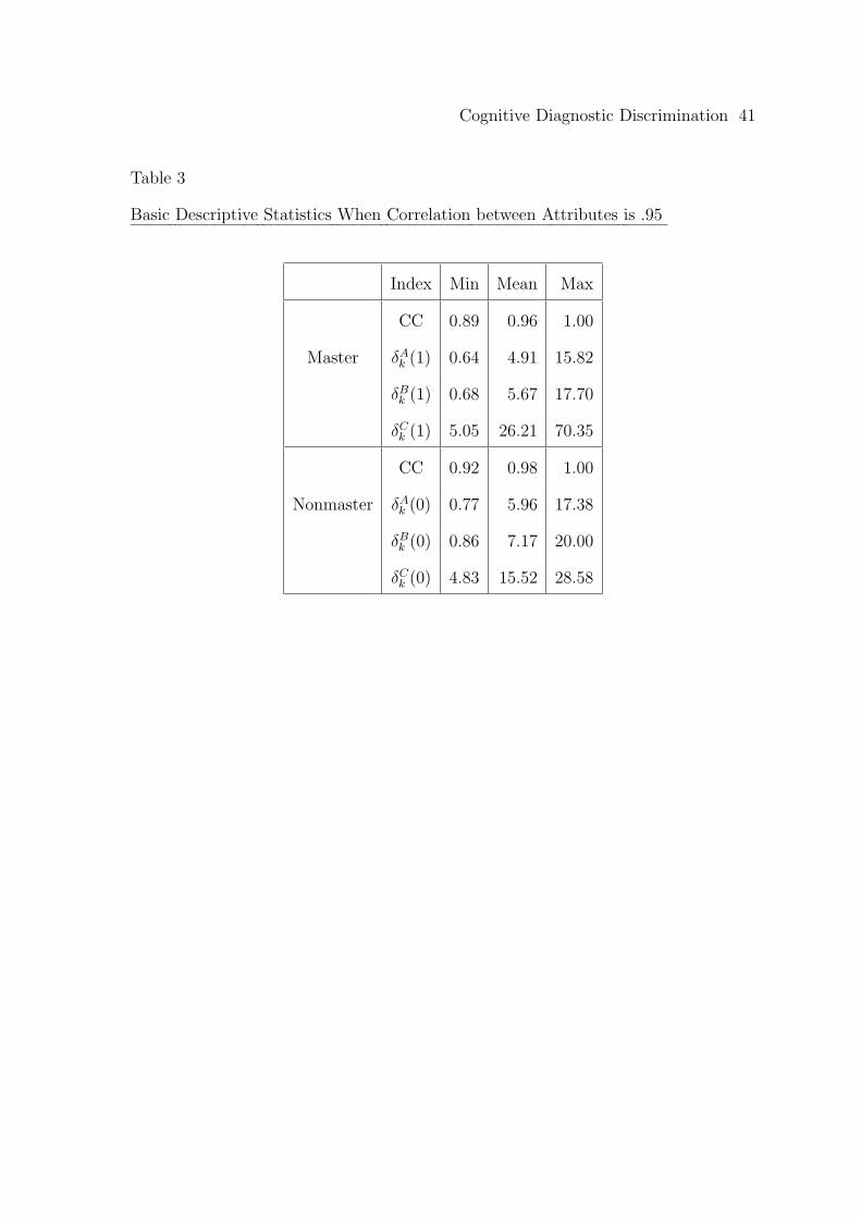
Table 3
Basic Descriptive Statistics When Correlation between Attributes is .95
Index Min Mean Max
CC 0.89 0.96 1.00
Master δAk (1) 0.64 4.91 15.82
δBk (1) 0.68 5.67 17.70
δCk (1) 5.05 26.21 70.35
CC 0.92 0.98 1.00
Nonmaster δAk (0) 0.77 5.96 17.38
δBk (0) 0.86 7.17 20.00
δCk (0) 4.83 15.52 28.58
Page 42
Cognitive Diagnostic Discrimination 42
Table 4
Correlation between the Discrimination Indices and Correct Classification
Study ρA ρB ρC
Att Cor .5 0.87 0.86 0.82
Masters Att Cor .75 0.87 0.85 0.80
Att Cor .95 0.85 0.83 0.79
Study ρA ρB ρC
Att Cor .5 0.90 0.90 0.94
Non-Masters Att Cor .75 0.88 0.88 0.93
Att Cor .95 0.83 0.83 0.89
Page 43
Cognitive Diagnostic Discrimination 43
Table 5
Correlation between the Transformed Discrimination Indices and Correct
Classification
Study ρA ρB ρC
Att Cor .5 0.97 0.97 0.97
Masters Att Cor .75 0.95 0.94 0.89
Att Cor .95 0.93 0.92 0.87
Study ρA ρB ρC
Att Cor .5 0.95 0.94 0.90
Non-Masters Att Cor .75 0.96 0.96 0.96
Att Cor .95 0.93 0.92 0.92
Page 44
Cognitive Diagnostic Discrimination 44
Figure Captions
Figure 1. Scatter plots of the Discrimination Indices with Correct Classification for
Masters
Figure 2. Scatter plots of the Discrimination Indices with Correct Classification for
Nonmasters
Figure 3. Scatter plots of the Transformed Discrimination Indices with Correct
Classification for Masters
Figure 4. Scatter plots of the Transformed Discrimination Indices with Correct
Classification for Nonmasters
Figure 5. Discrimination Indices with Correct Classification for Masters in High
Correlation Example
Figure 6. Discrimination Indices with Correct Classification for Nonmasters in High
Correlation Example
Page 45
Cognitive Diagnostic Discrimination, Figure 1
0 10 200.7
0.8
0.9
1Reliability Index A
Sim
ulat
ion
with
Cor
r .5
0 10 200.7
0.8
0.9
1Reliability Index B
0 20 40 600.7
0.8
0.9
1Reliability Index C
0 5 10 150.8
0.85
0.9
0.95
1
Sim
ulat
ion
with
Cor
r .7
5
0 10 200.8
0.85
0.9
0.95
1
0 20 40 600.8
0.85
0.9
0.95
1
0 10 200.9
0.95
1
Sim
ulat
ion
with
Cor
r .9
5
0 10 200.9
0.95
1
0 50 1000.9
0.95
1
Page 46
Cognitive Diagnostic Discrimination, Figure 2
0 10 200.7
0.8
0.9
1Reliability Index A
Sim
ulat
ion
with
Cor
r .5
0 10 20 300.7
0.8
0.9
1Reliability Index B
0 10 20 300.7
0.8
0.9
1Reliability Index C
0 10 200.8
0.85
0.9
0.95
1
Sim
ulat
ion
with
Cor
r .7
5
0 10 200.8
0.85
0.9
0.95
1
0 10 20 300.8
0.85
0.9
0.95
1
0 10 200.92
0.94
0.96
0.98
1
Sim
ulat
ion
with
Cor
r .9
5
0 10 200.92
0.94
0.96
0.98
1
0 10 20 300.92
0.94
0.96
0.98
1
Page 47
Cognitive Diagnostic Discrimination, Figure 3
−2 0 2 40.7
0.8
0.9
1Reliability Index A
Sim
ulat
ion
with
Cor
r .5
−2 0 2 40.7
0.8
0.9
1Reliability Index B
1 2 3 40.7
0.8
0.9
1Reliability Index C
−2 0 2 40.8
0.85
0.9
0.95
1
Sim
ulat
ion
with
Cor
r .7
5
−2 0 2 40.8
0.85
0.9
0.95
1
1 2 3 40.8
0.85
0.9
0.95
1
−2 0 2 40.9
0.95
1
Sim
ulat
ion
with
Cor
r .9
5
−2 0 2 40.9
0.95
1
0 2 4 60.9
0.95
1
Page 48
Cognitive Diagnostic Discrimination, Figure 4
−2 0 2 40.7
0.8
0.9
1Reliability Index A
Sim
ulat
ion
with
Cor
r .5
−2 0 2 40.7
0.8
0.9
1Reliability Index B
1 2 3 40.7
0.8
0.9
1Reliability Index C
−2 0 2 40.8
0.85
0.9
0.95
1
Sim
ulat
ion
with
Cor
r .7
5
−2 0 2 40.8
0.85
0.9
0.95
1
1 2 3 40.8
0.85
0.9
0.95
1
−2 0 2 40.92
0.94
0.96
0.98
1
Sim
ulat
ion
with
Cor
r .9
5
0 1 2 30.92
0.94
0.96
0.98
1
1 2 3 40.92
0.94
0.96
0.98
1
Page 49
Cognitive Diagnostic Discrimination, Figure 5
−1 0 10.8
0.85
0.9
0.95
1Reliability Index A
Attr
ibut
e 1
−1 0 10.8
0.85
0.9
0.95
1Reliability Index B
0 5 10 150.8
0.85
0.9
0.95
1Reliability Index C
0 10 20 300.85
0.9
0.95
1
Attr
ibut
e 2
0 10 20 300.85
0.9
0.95
1
0 10 20 300.85
0.9
0.95
1
Page 50
Cognitive Diagnostic Discrimination, Figure 6
−1 0 10.8
0.85
0.9
0.95
1Reliability Index A
Attr
ibut
e 1
−1 0 10.8
0.85
0.9
0.95
1Reliability Index B
0 10 200.8
0.85
0.9
0.95
1Reliability Index C
0 20 400.8
0.85
0.9
0.95
1
Attr
ibut
e 2
0 20 400.8
0.85
0.9
0.95
1
0 20 400.8
0.85
0.9
0.95
1