An investigation into the factors influencing thedetectability of oil spills using spectral indices inan oil-polluted environment
Bashir Adamu, Kevin Tansey & Booker Ogutu
To cite this article: Bashir Adamu, Kevin Tansey & Booker Ogutu (2016) An investigationinto the factors influencing the detectability of oil spills using spectral indices in an oil-polluted environment, International Journal of Remote Sensing, 37:10, 2338-2357, DOI:10.1080/01431161.2016.1176271
To link to this article: http://dx.doi.org/10.1080/01431161.2016.1176271
An investigation into the factors influencing the detectabilityof oil spills using spectral indices in an oil-pollutedenvironmentBashir Adamua,b, Kevin Tanseya and Booker Ogutuc
aDepartment of Geography, University of Leicester, Leicester, UK; bDepartment of Geography, ModibboAdama University of Technology, Yola, Nigeria; cDepartment of Geography, University of Southampton,Southampton, UK
ABSTRACTThe aim of this article is to investigate and test the influence of oilspill volume and time gap (number of days between oil spillevents and image acquisition date) on normalized difference vege-tation index (NDVI) and normalized difference water index (NDWI).This was carried out to determine the effect of these factors onvegetation condition affected by the oil spill. Based on regressionanalysis, it was shown that increase in the volume of oil spillresulted in increased deterioration of vegetation condition (esti-mated using NDVI and NDWI) in the study site. The study alsotested how the length of time gap between the oil spill and imageacquisition date influences the detectability of impacts of oil spillon vegetation. The results showed that the length of timebetween image acquisition and oil spill influenced the detectabil-ity of impacts of oil spill on vegetation condition. The longer thetime between the date of image acquisition and the oil spill event,the lower the detectability of impacts of oil spill on vegetationcondition. The NDVI seemed to produce better results than theNDWI. In conclusion, time and volume of oil spill can be importantfactors influencing the detection of pollution using vegetationindices (VIs) in an oil-polluted environment.
ARTICLE HISTORYReceived 2 October 2015Accepted 25 March 2016
1. Introduction
Oil has become a vital commodity for the government as a source of revenue andnational economic growth (Bridge 2008). It also serves as a source of energy for themaintenance of industrial civilization, which has become a critical concern for manycountries (Smil 2010). Globally, energy consumption in almost all regions of the worldhas increased from 1965 to 2010 and likewise the crude oil production (IEA 2011; BP2011). The increase in oil production has undoubtedly continued to add pressure on thenatural and human environment. The consequences for oil production and pollutionfrom the oil operation have been documented around the world. Oil spills occurringduring the exploration, production, and distribution/transportation of crude oil can havea disastrous impact on the environment. When oil spill occurs, it degrades the air quality
CONTACT Bashir Adamu [email protected] Department of Geography, University of Leicester, Leicester, UK
INTERNATIONAL JOURNAL OF REMOTE SENSING, 2016VOL. 37, NO. 10, 2338–2357http://dx.doi.org/10.1080/01431161.2016.1176271
due to emission, and leads to loss of vegetation and soil productivity (Obire andNwaubeta 2002). Frequent incidences of oil spills have had wide-ranging impacts,including the contamination of streams and rivers, forest destruction, and loss ofbiodiversity. There have been several incidents of oil spills in places such as the Gulfof Mexico in 2010, Canadian marine waters (Serra-Sogas et al. 2008) and Prince WilliamsSound, off the coast of Alaska in March 1989. According to Exxon Mobil the total volumeof hydrocarbons spilled on soil and water was 9,100 barrels (bbl) in 2014 from differentincidences. In another incident, in 1989 the Exxon Valdez reported by Exxon Mobil in2003 that a super-tanker ran aground at Alaska’s Prince William Sound and dischargedmore than 250,000 bbl of oil into the environment (Short 2003). The European EconomicCommunity (EEA) also reported in 2007 that primary pollutants such as heavy metalsand mineral oil caused 37.3% and 33.7% soil contamination, respectively. In other partsof the world, for instance, Nigeria, Colombia, Peru, Ecuador, and Bolivia, substantial oiloperations are located in the rain forest. As such, oil extraction and transportation canbe destructive to the natural environment. Oil spills from burst pipelines and toxicdrilling by-products may be dumped directly into local channels and rivers (CIA 2005).Oil spills in water may severely affect the marine environment, causing a decline inphytoplankton and other aquatic organisms (Jha, Levy, and Gao 2008). The multipliereffect of this environmental destruction will result in the deterioration of the environ-ment through the depletion of resources such as air, water, vegetation and soils, the lossof ecosystems, and the extinction of wildlife. Oil spill site characterization traditionallyrequires extensive field sampling and laboratory analysis (Slonecker et al. 2010). Fielddata collection is expensive and time-consuming, making this approach unsustainable.Remote sensing offers an efficient, time-saving, cost-effective, and non-destructivemethod of characterizing oil spills and their impacts on the environment.
Remote sensing has an advantage of covering large oil-polluted areas and can accessinformation on environmental variables affected by pollution through their spatial andspectral characteristics. Furthermore, remote sensing offers the capacity to acquire datain remote areas that are difficult to access. The use of remote sensing for oil orhydrocarbon pollution monitoring dates back to the 1970s, where aerial photographswere used for the first time (Casciello et al. 2007). There are a number of studies thatdemonstrate the use of remote sensing for the detection of oil pipelines and vegetationstress from oil pollution, quantification of pollution/stress level, and monitoring afterremediation (van der Werff et al. 2008). Remote-sensing sensors that record informationin the ultraviolet (UV), thermal infrared, and microwave sections of the electromagneticspectrum have been used to detect oil spills (Brekke and Solberg 2005; Zhao and Li2007). Studies have shown that hyperspectral sensors, e.g. Airborne Visible/InfraredImaging Spectrometer (AVARIS) and Airborne Imaging Spectrometer for Application(AISA), have capabilities to detect oil spill (Jha, Levy, and Gao 2008; Landgrebe 2005).Data from active sensors that collect data in radio wavelength have also been used todetect the presence of oil in offshores areas mainly through the reduction of oceanreflectance (Brown and Fingas 2003). Microwave sensors have been used to detect oilspill and their thickness (Jha, Levy, and Gao 2008), whereas laser-acoustic oil thicknesssensors have been used to detect oil mechanical properties instead of its optical andelectromagnetic properties (Goodman 1994). Onshore oil pollution monitoring inforested areas using remote-sensing data has been limited, especially in developing
INTERNATIONAL JOURNAL OF REMOTE SENSING 2339
Dow
nloa
ded
by [
Uni
vers
ity o
f L
eice
ster
] at
08:
28 0
3 Ju
ne 2
016
countries such as Nigeria, mainly due to the lack of readily available data. The recentrelease of all Landsat archive of images has made it possible to explore the use of theseimages to monitor the impacts of onshore oil spills on vegetation condition in devel-oping countries such as Nigeria.
Monitoring the impacts of oil spills on vegetation using remote-sensing data requiresan understanding of the spectral reflectance characteristics of vegetation. Vegetationhas a unique spectral signature that enables it to be distinguishable from other types ofland cover in an optical/near-infrared (NIR) image. Vegetation has reflectance in bothblue and red regions of the spectrum because of the absorption of chlorophyll forphotosynthesis and the relatively high reflectance at the green region (Sims 2002).Furthermore, in the NIR region, vegetation has a high reflectance mostly due to thecellular structure in the leaves (Purkis and Klemas 2011). Therefore, vegetation and itscondition can be characterized using reflectance information form the NIR and thevisible bands. The common approach of carrying this out is to calculate the band ratiosoften referred to as vegetation indices (VIs) and monitor their dynamics. Healthy plantshave diagnostic high reflectance in the NIR region and low reflectance in the visiblebands and hence the high values of VIs indicate healthy vegetation and vice versa. It hasbeen suggested that the presence of hydrocarbons seems to produce a change in theinternal structure of the plant that results in low reflectance values and oil pollution mayalso lead to low density of vegetation in the affected areas (Oliveira, Crosta, andGoncalves 1997). In addition, vegetation growing near leaking gas pipelines has beenshown to have changes in their geobotany and reflectance (van der Meer et al. 2002;Arellano et al. 2015). The geobotanical anomalies were associated with the effects of oilspills and pollution on the growth of the vegetation (Noomen et al. 2008). Furthermore,changes in the colour of leaves, stems, and trunks are an extremely good indication ofplants’ response to stress from oil pollution (Guyot, Baret, and Jacquemoud 1992). Allthese changes due to oil spills and pollution manifest themselves in the VIs; hence, theimpacts of oil pollution on vegetation condition can be assessed using VIs. VIs (e.g.normalized difference vegetation index, NDVI) have shown a great potential for detect-ing the impacts of oil pollution on vegetation in oil-polluted environments (Zhu et al.2013; Adamu, Tansey, and Ogutu 2015). In an earlier study, Adamu, Tansey, and Ogutu(2015) showed that oil spills resulted in the reduction of values of VIs (especially theNDVI and the normalized difference water index, NDWI), implying these indices can beused to detect the impacts of oil pollution on vegetation condition. However, in thatstudy, factors that influence the detectability of impacts of oil pollution on vegetationusing the spectral indices (e.g. volume of oil spill and time difference between spill andimage acquisition) were not investigated.
A number of factors can influence the detectability of impacts of oil spill on vegeta-tion condition. One such factor is the toxicity of the oil spilled, i.e. the higher the toxicity,the higher the impacts on vegetation (Reed et al. 1999; Lehr 2001; Mendelssohn et al.2012). A second factor that influences the impacts of oil spill on vegetation is the volumeof oil spill. Noomen et al. (2012) suggested that high volumes of oil spill in vegetatedareas might result in shortage of oxygen supply to plants and consequently retard theirgrowth. Furthermore, Pezeshki et al. (2000) demonstrated how a large volume of oilspills can impact vegetation more than the small spills. Therefore, it is expected thathigh-volume spills would lead to higher impacts on the vegetation condition as it will
2340 B. ADAMU ET AL.
Dow
nloa
ded
by [
Uni
vers
ity o
f L
eice
ster
] at
08:
28 0
3 Ju
ne 2
016
take time for larger-volume spills to degrade and evaporate (Mendelssohn et al. 2012).Finally, the length of time between the spill event and the image acquisition may affectthe detectability of oils spills from remote-sensing data. As mentioned previously, oilspills degrade and evaporate with time and hence if the imagery is acquired at a longerlength of time from the spill date, the vegetation in the area may already haverecovered, making it difficult to detect the impacts of the oil spill. A study by Yimet al. (2011) showed that samples of oil residue collected 90–120 days after pollutionalready had the molecular weight of their alkanes depleted or biodegraded. Duke et al.(2000) observed that obvious signs of stress of mangrove plants were noticed within thefirst two weeks of oil spill, causing chlorosis to defoliation to death of the affected plants.This study aims to investigate the influence of volume and time of image acquisition inthe detectability of oil spill impacts of vegetation in the Niger Delta, Nigeria, using twoindices (i.e. the NDVI and NDWI). The indices (NDVI and NDWI) used in the study areproducts derived from atmospherically corrected and temporarily processed Landsatimages to further reduce noise. In brief the NDWI uses infrared channels (NIR and MIR)centred approximately at 0.86 and 1.24 µm, and primarily sensitive to the liquid contentof vegetation from space (Gao 1996). NDVI uses a formula based on the fact thatchlorophyll absorbs RED, whereas the mesophyll leaf structure scatters NIR (Myneniet al. 2002).
2. Study area
2.1. Physical environment
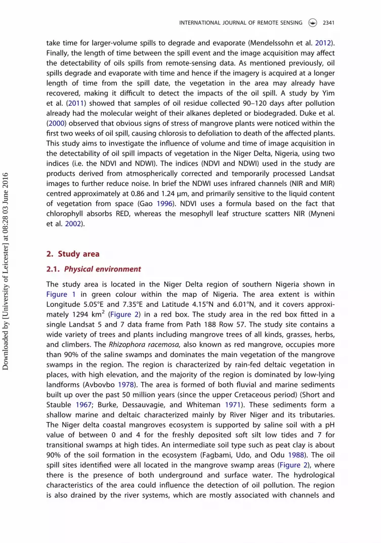
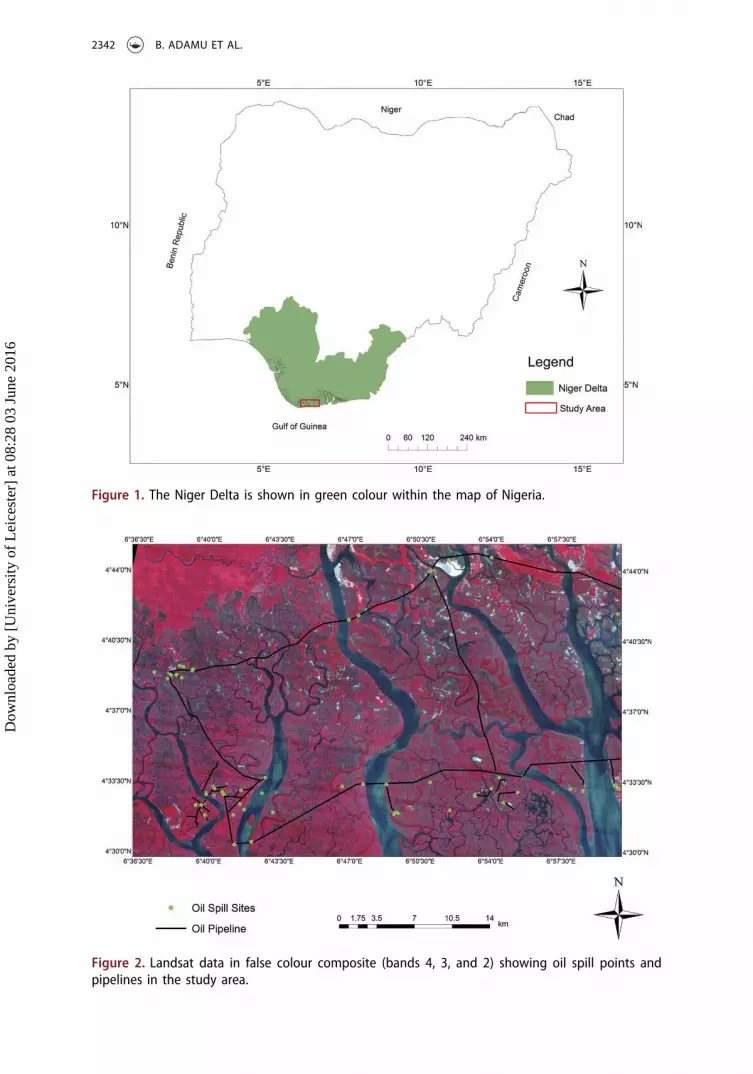
The study area is located in the Niger Delta region of southern Nigeria shown inFigure 1 in green colour within the map of Nigeria. The area extent is withinLongitude 5.05°E and 7.35°E and Latitude 4.15°N and 6.01°N, and it covers approxi-mately 1294 km2 (Figure 2) in a red box. The study area in the red box fitted in asingle Landsat 5 and 7 data frame from Path 188 Row 57. The study site contains awide variety of trees and plants including mangrove trees of all kinds, grasses, herbs,and climbers. The Rhizophora racemosa, also known as red mangrove, occupies morethan 90% of the saline swamps and dominates the main vegetation of the mangroveswamps in the region. The region is characterized by rain-fed deltaic vegetation inplaces, with high elevation, and the majority of the region is dominated by low-lyinglandforms (Avbovbo 1978). The area is formed of both fluvial and marine sedimentsbuilt up over the past 50 million years (since the upper Cretaceous period) (Short andStauble 1967; Burke, Dessauvagie, and Whiteman 1971). These sediments form ashallow marine and deltaic characterized mainly by River Niger and its tributaries.The Niger delta coastal mangroves ecosystem is supported by saline soil with a pHvalue of between 0 and 4 for the freshly deposited soft silt low tides and 7 fortransitional swamps at high tides. An intermediate soil type such as peat clay is about90% of the soil formation in the ecosystem (Fagbami, Udo, and Odu 1988). The oilspill sites identified were all located in the mangrove swamp areas (Figure 2), wherethere is the presence of both underground and surface water. The hydrologicalcharacteristics of the area could influence the detection of oil pollution. The regionis also drained by the river systems, which are mostly associated with channels and
INTERNATIONAL JOURNAL OF REMOTE SENSING 2341
Dow
nloa
ded
by [
Uni
vers
ity o
f L
eice
ster
] at
08:
28 0
3 Ju
ne 2
016
Figure 1. The Niger Delta is shown in green colour within the map of Nigeria.
Figure 2. Landsat data in false colour composite (bands 4, 3, and 2) showing oil spill points andpipelines in the study area.
2342 B. ADAMU ET AL.
Dow
nloa
ded
by [
Uni
vers
ity o
f L
eice
ster
] at
08:
28 0
3 Ju
ne 2
016
streams. The surface water, freshwater, and deltaic estuaries (an area of interactionbetween freshwater and seawater) cover approximately 2,370 km2 and stagnantswamp 8600 km2 spanning an area of 1900 km2, and other sources of inflow duringthe rainy season, which is also influenced by tidal variations. The width and velocityof freshwater channels increase downstream to meandering or braided channels inthe delta.
2.2. Climate
Nigeria’s climate is tropical, characterized by high temperatures and humidity as well asmarked wet and dry seasons, although there are variations from South to North. Thetotal rainfall decreases from the coast northwards (Oguntunde, Abiodun, and Lischeid2011). The long wet season starts in March and lasts to the end of July, with a peakperiod in June over most parts of Niger Delta similar to other parts of southern Nigeria. Itis a period of thick clouds and is excessively wet particularly in the Niger Delta and thecoastal lowlands. The long dry season period starts from late October and lasts to earlyMarch with peak dry conditions between early December and late February (Adejuwon2012). The annual temperature in the Niger Delta ranges between 26oC and 34oC, withthe highest during the dry season (November–March) and the lowest between 24.5oCand 26.9oC in June, July, and August. The topography of the Niger Delta or Nigeriancoastal areas is generally low-lying at about 2–4 m above the sea level (Allen 1965; Ajao,Oyewo, and Unyimadu 1996), which is also a factor that could influence the flowdirection of the oil spilt in the study.
2.3. Land use and land cover
The coast of Nigeria’s Niger Delta region where the study area is located is characterizedby a high concentration of oil exploration and local farming activities. This has led tocontinuous changes in both land-cover and land-use patterns of the region. It has alsobeen shown that expansion in the oil exploration and exploitation activities hadincreased pressure with heavy impact on the natural ecosystems as a result of oil spillincidences (Abbas 2012). Records have shown that most of the oil pollution from oiloperations in the regions has remained in the environment for many years withoutclean-up and yet to recover the lost natural vegetation (UNEP 2011).
3. Data analysis
The oil spill events for 56 oil spill sites were recorded in 1985, 1986, 1998, 1999, 2000,2004, 2006, and 2007 with the volume of oil spill ranging between 3 and 3500 bbl(Table 1). The 56 sample spill sites analysed in the study were all located within the samevegetation type (swamp mangrove forest) to ensure that there are no significant varia-tions in the vegetation spectral reflectance. Note in this study, the volume of oil spill isquantified in bbl and interpreted using SI units as 1 bbl approximately 160 litres (l).
The ancillary data used include oil pipeline maps, spill records from 1985 to 2006containing information on the date of events, vegetation land-cover type, causes of spill,and GPS locations of spill points (showing where the oil spill events occurred) obtained
INTERNATIONAL JOURNAL OF REMOTE SENSING 2343
Dow
nloa
ded
by [
Uni
vers
ity o
f L
eice
ster
] at
08:
28 0
3 Ju
ne 2
016
from Shell Nigeria through the Department of Petroleum Resources, Nigeria (DPRN,Nigeria’s oil and gas regulatory agency).
3.1. Data preprocessing
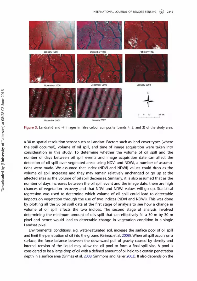
In this article Landsat TM and ETM data obtained as digital number (DN) were convertedto comparable measures of radiance and reflectance as a starting point for dataprocessing. Thus, the images were processed by converting top-of-atmosphere radiancevalues to surface reflectance following a method proposed by Chander, Markham, andHelder (2009). The Fast Line-of-sight Atmospheric Analysis of Spectral Hypercubes(FLAASH) routine available on the Exelis Environment Visual Information (ENVI) softwarewas used to change the radiance values into surface reflectance. Atmospheric correctionwas then performed on the reflectance values derived using the FLAASH routine. Theinput file was converted to radiance image in a band-interleaved-by-line (BIL) formatwith a scale factor of 1.0 (μW cm–2 sr–1 nm–1) before applying the FLAASH module. TheFLAASH module input information (such as flight date and time, sensor altitude, andsensor location) needed for the processing of these images was contained in theLandsat image metadata file downloaded from the USGS archive. Sensor altitude (km)is automatically set according to sensor type and the average study area elevation(0.4 km) was used as an input for ground elevation. Some multispectral sensors suchas Landsat data do not have appropriate bands to perform water retrieval; hence, thiswas not undertaken in this work. Figure 3 shows the preprocessed Landsat 5 and 7images used for the analysis.
3.2. Method of analysis
From the database, the range of volume of oil spill that occurred in the study is from aminimum of 3 to a maximum of 3500 bbl and the number of days computed betweenthe oil spill event and image acquisition date ranges from 2 to 844 days. The relationshipbetween oil spill volume and the level of impact on the vegetation health has beendemonstrated in Mackay and Matsugu (1973) and Mackay and Mohtadi (1975) inCanada. Hypothetically, a small volume of oil spill over land may occupy little space ina pixel of 30 m resolution. In contrast, the large volume of oil spill could occupy a largespace in a 30 m pixel over land. Thus, it is expected that a smaller volume of oil spill mayhave little impact on vegetation, thereby limiting the detectability of these effects using
Table 1. Year of oil spills, sample points, and available image data.Year of Spill Sample Points Acquisition Date
1985 2 17 January 19861986 9 19 December 19861998 7 21 February 19871999 11 29 November 19992000 10 17 December 20002002 6 8 January 20032004 4 26 November 20042006 5 19 January 20072007 1 19 January 2007Total 56
2344 B. ADAMU ET AL.
Dow
nloa
ded
by [
Uni
vers
ity o
f L
eice
ster
] at
08:
28 0
3 Ju
ne 2
016
a 30 m spatial resolution sensor such as Landsat. Factors such as land-cover types (wherethe spill occurred), volume of oil spill, and time of image acquisition were taken intoconsideration in this study. To determine whether the volume of oil spill and thenumber of days between oil spill events and image acquisition date can affect thedetection of oil spill over vegetated areas using NDVI and NDWI, a number of assump-tions were made. We assumed that index (NDVI and NDWI) values could drop as thevolume oil spill increases and they may remain relatively unchanged or go up at theaffected sites as the volume of oil spill decreases. Similarly, it is also assumed that as thenumber of days increases between the oil spill event and the image date, there are highchances of vegetation recovery and that NDVI and NDWI values will go up. Statisticalregression was used to determine which volume of oil spill could lead to detectableimpacts on vegetation through the use of two indices (NDVI and NDWI). This was doneby plotting all the 56 oil spill data at the first stage of analysis to see how a change involume of oil spill affects the two indices. The second stage of analysis involveddetermining the minimum amount of oils spill that can effectively fill a 30 m by 30 mpixel and hence would lead to detectable change in vegetation condition in a singleLandsat pixel.
Environmental conditions, e.g. water-saturated soil, increase the surface pool of oil spilland limit the penetration of oil into the ground (Grimaz et al. 2008). When oil spill occurs on asurface, the force balance between the downward pull of gravity caused by density andinternal tension of the liquid may allow the oil pool to form a final spill size. A pool isconsidered to be a large drop of oil with a defined amount of oil held to a certain penetrationdepth in a surface area (Grimaz et al. 2008; Simmons and Keller 2003). It also depends on the
Figure 3. Landsat-5 and -7 images in false colour composite (bands 4, 3, and 2) of the study area.
INTERNATIONAL JOURNAL OF REMOTE SENSING 2345
Dow
nloa
ded
by [
Uni
vers
ity o
f L
eice
ster
] at
08:
28 0
3 Ju
ne 2
016
property of the oil (in the case for this study, heavy oils are used as no specific oil type isconsidered); the spilled oil will eventually stand a certain height or depth above the surface(Simmons, Keller, and Hylden 2004). For example this model (Simmons, Keller, and Hylden2004) presumed that the volume of oil-spilled partition over an area is given by
V ¼ Aδφþ Ah; (1)
where h is the height of liquid standing above the surface. Liquid below penetrated to acertain depth, δ, in the substrate porosity, φ. Thus the height is given by
1� cosθð Þ � σ ¼ ρ� g� h2; (2)
where h = spill height (cm)ρ = density (gm/ml)g = gravity accelerationσ = surface tension (dyne/cm)θ = contact angle (angle between spill height of liquid and surface)Oil spill height can be determined by surface tension divided by the weight density of
liquid for adhesion quantified by contact angle. In Simmons, Keller, and Hylden (2004)the model used different types of oil liquid properties to produce different heights of oilspill based on various scenarios ranging from 0.01 to 0.5 cm. Since the oil found in theNiger Delta could be assumed to behave similar to the ones demonstrated, the height ofoil spill is presumed at 0.04 m for this study based on the calculation in Simmons, Keller,and Hylden (2004). The following calculation was used to predict the expected volumeof oil spill to fill a 30 m pixel:
Consequently, in further analysis, 225 bbl was used as the minimum value whereimpacts of oil pollution on vegetation can be detected.
In the second part of the analysis, the influence of the number of days between oilspill and date of image acquisition on the detectability of pollution impacts on vegeta-tion was determined. In the first stage of this analysis, all the date data was used toderive the regression statistics between time and the VIs. Next, the data was divided intotwo dates (i.e. 0–1 year and 1–2 years) to determine any variations in vegetationresponse.
2346 B. ADAMU ET AL.
Dow
nloa
ded
by [
Uni
vers
ity o
f L
eice
ster
] at
08:
28 0
3 Ju
ne 2
016
4. Results
The data in Table 2 shows that some spill sites have high values of NDVI and NDWIdespite a large volume of spills; others appear to have a low volume of spill but withhigh values of NDVI and NDWI.
4.1. Influence of volume of oil spill on NDVI and NDWI
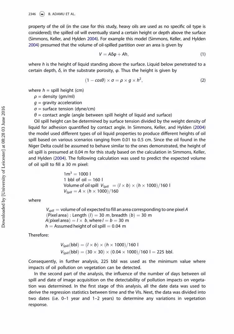
The computed NDVI and NDWI from all the 56 sample sites in Table 2 were used todetermine the relationship between the indices and the volume of oil spill using all thedata in Table 2. All the oil spill data (volume of oil spill) were plotted against NDVI andNDWI in Figure 4.
The relationship between the two indices and the volume of oil spill between 3 and3500 bbl indicated was weak, with the coefficient of determination (R2 = 0.0001 andR2 = 0.02) for NDVI and NDWI, respectively (Figures 4(a) and 4(b), respectively). Thereason for this analysis is to determine whether there is any relationship at all betweenall the volume of oil spill data and the spectral indices without considering the influenceof the number of days between the oil spill events and the image acquisition date.Generally, considering the regression analysis shows that the volume of oil spill indi-cated a poor relationship with the NDVI and NDWI at this stage. The next stage ofanalysis used a minimum volume of 225 bbl calculated in the methods section to
Table 2. Number of sample points, volume of oil spill, and time gap between oil spill and imagedates.SamplePoints
Volume Ofoil (bbl) Time (Days) NDVI NDWI Sample Points Volume Time (Days) NDVI NDWI
determine whether there would be any improvement in the detection of the influenceof volume of oil spill on the VIs. This amount of oil spill was assumed capable of coveringa single Landsat pixel and hence would result in detectable changes in vegetationcondition.
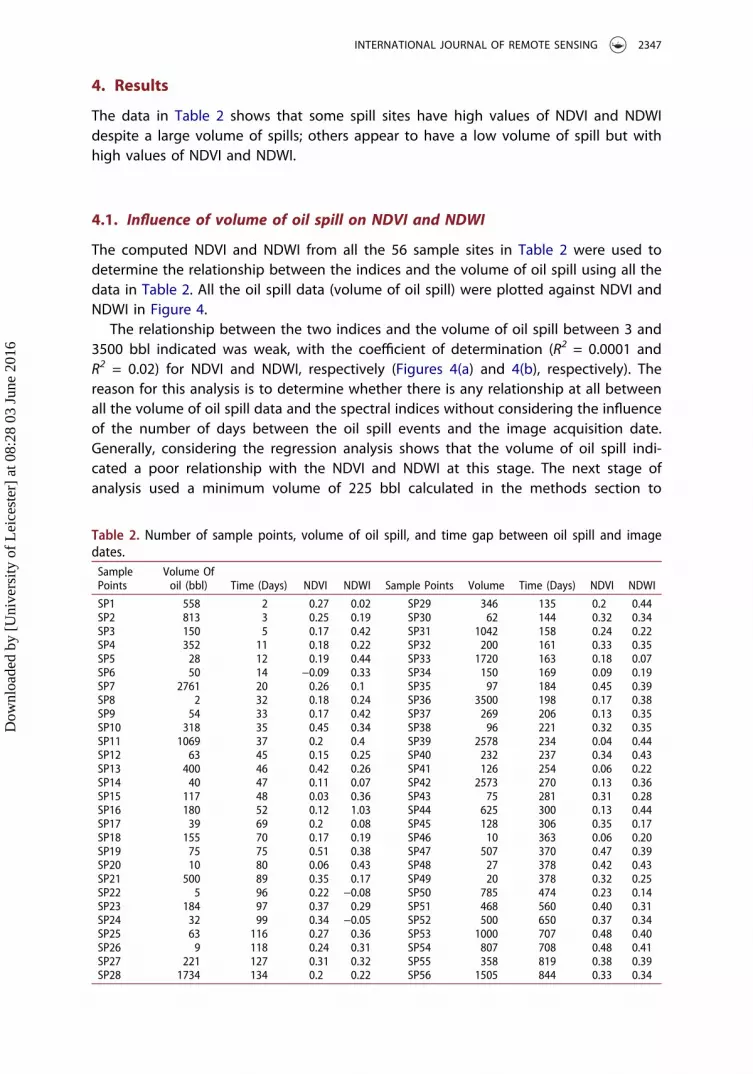
Figure 5 shows the relationship between oil spill and the two VIs when the minimumvolume of 225 bbl is used. In this figure the relationship between the volume of oil spill(> 225 bbl) and the two indices (NDVI and NDWI) was better than the one shown inFigure 4. Figure 5 shows that as the volume increases, the VIs value decrease. This wasmore pronounced in the NDVI than in the NDWI.
To further analyse the relationship between the oil spill volume and the VIs, the oilspill volumes were divided into different categories (i.e. 225–400 bbl, 401–1000 bbl, and
(a) (b)
y = -1x10⁻⁴-06x + 0.2296R² = 0.0001
0.20
0.10
0.00
0.10
0.20
0.30
0.40
0.50
0.60
ND
VI
Volume of Oil (bbl)
y = -1x10⁻³-05x + 0.2571R² = 0.0207
0.20
0.10
0.00
0.10
0.20
0.30
0.40
0.50
0 1000 2000 3000 40000 1000 2000 3000 4000
ND
WI
Volume of Oil (bbl)
Figure 4. Relationship between NDVI and NDWI and all volumes of oil spill.
(a) (b)
y = -1x10⁻⁶-05x + 0.3464R² = 0.2255
0
0.1
0.2
0.3
0.4
0.5
0.6
ND
VI
Volume of oil (bbl)
y = -1x10⁻¹-05x + 0.312R² = 0.0062
0
0.05
0.1
0.15
0.2
0.25
0.3
0.35
0.4
0.45
0.5
0 1000 2000 3000 4000 0 1000 2000 3000 4000
ND
WI
Volume of oil (bbl)
Figure 5. Relationship between (a) NDVI and (b) NDWI and volume of oil spill where the volume wasgreater than 225 bbl.
2348 B. ADAMU ET AL.
Dow
nloa
ded
by [
Uni
vers
ity o
f L
eice
ster
] at
08:
28 0
3 Ju
ne 2
016
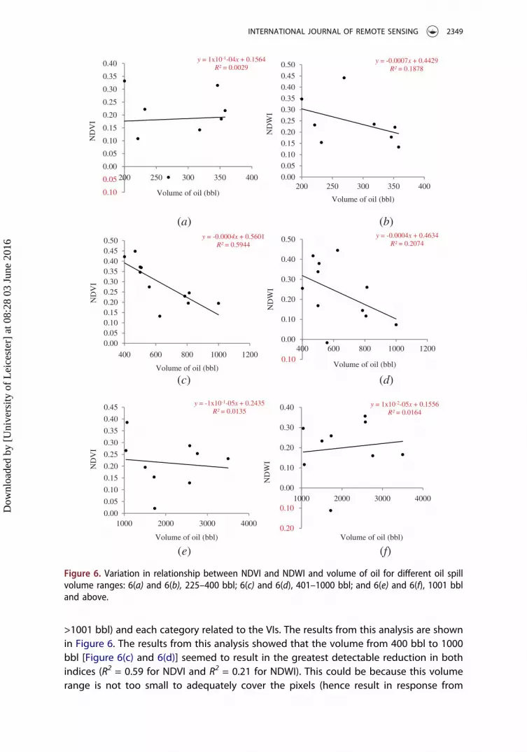
>1001 bbl) and each category related to the VIs. The results from this analysis are shownin Figure 6. The results from this analysis showed that the volume from 400 bbl to 1000bbl [Figure 6(c) and 6(d)] seemed to result in the greatest detectable reduction in bothindices (R2 = 0.59 for NDVI and R2 = 0.21 for NDWI). This could be because this volumerange is not too small to adequately cover the pixels (hence result in response from
y = 1x10⁻¹-04x + 0.1564R² = 0.0029
0.10
0.05
0.00
0.05
0.10
0.15
0.20
0.25
0.30
0.35
0.40
ND
VI
Volume of oil (bbl)
y = -0.0007x + 0.4429R² = 0.1878
0.00
0.05
0.10
0.15
0.20
0.25
0.30
0.35
0.40
0.45
0.50
ND
WI
Volume of oil (bbl)
y = -0.0004x + 0.5601R² = 0.5944
0.000.050.100.150.200.250.300.350.400.450.50
ND
VI
Volume of oil (bbl)
y = -0.0004x + 0.4634R² = 0.2074
0.10
0.00
0.10
0.20
0.30
0.40
0.50
ND
WI
Volume of oil (bbl)
y = -1x10⁻¹-05x + 0.2435R² = 0.0135
0.00
0.05
0.10
0.15
0.20
0.25
0.30
0.35
0.40
0.45
ND
VI
Volume of oil (bbl)
y = 1x10⁻²-05x + 0.1556R² = 0.0164
0.20
0.10
0.00
0.10
0.20
0.30
0.40
200 250 300 350 400200 250 300 350 400
400 600 800 1000 1200400 600 800 1000 1200
1000 2000 3000 4000
1000 2000 3000 4000
ND
WI
Volume of oil (bbl)
(e) (f)
(c) (d)
(a) (b)
Figure 6. Variation in relationship between NDVI and NDWI and volume of oil for different oil spillvolume ranges: 6(a) and 6(b), 225–400 bbl; 6(c) and 6(d), 401–1000 bbl; and 6(e) and 6(f), 1001 bbland above.
INTERNATIONAL JOURNAL OF REMOTE SENSING 2349
Dow
nloa
ded
by [
Uni
vers
ity o
f L
eice
ster
] at
08:
28 0
3 Ju
ne 2
016
plants) and not too large to contaminate the reflectance of vegetation recorded bysatellite sensor (which would reduce the sensitivity of the VIs).
4.2. Analysis of influence of time on NDVI and NDWI
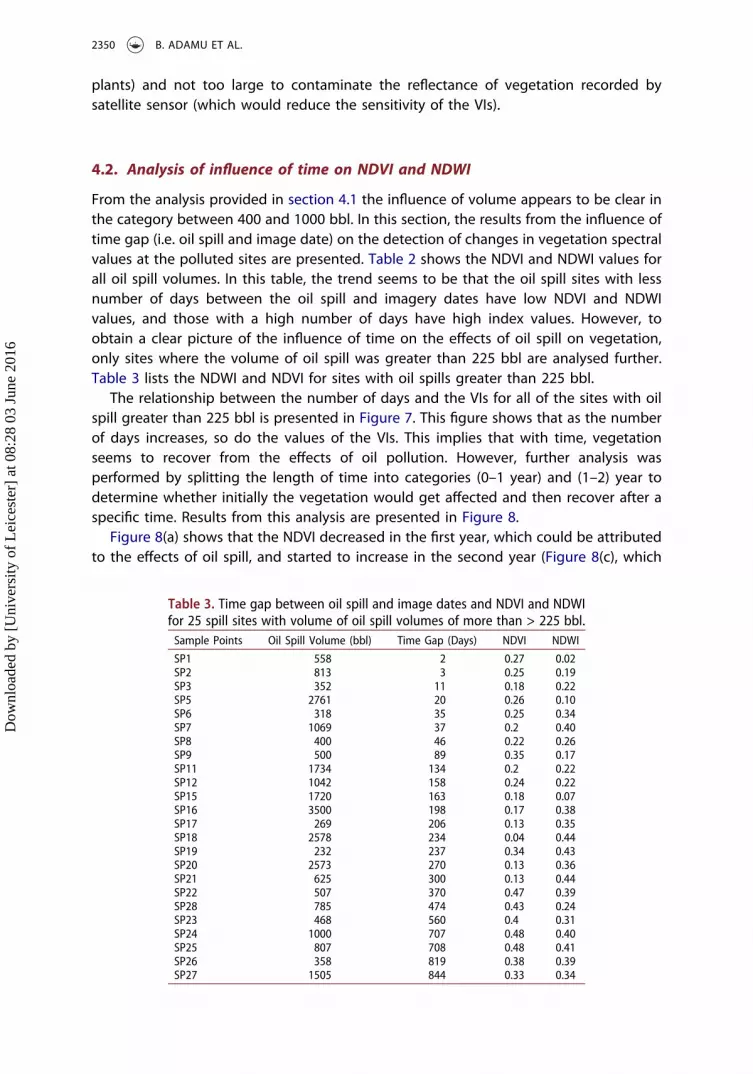
From the analysis provided in section 4.1 the influence of volume appears to be clear inthe category between 400 and 1000 bbl. In this section, the results from the influence oftime gap (i.e. oil spill and image date) on the detection of changes in vegetation spectralvalues at the polluted sites are presented. Table 2 shows the NDVI and NDWI values forall oil spill volumes. In this table, the trend seems to be that the oil spill sites with lessnumber of days between the oil spill and imagery dates have low NDVI and NDWIvalues, and those with a high number of days have high index values. However, toobtain a clear picture of the influence of time on the effects of oil spill on vegetation,only sites where the volume of oil spill was greater than 225 bbl are analysed further.Table 3 lists the NDWI and NDVI for sites with oil spills greater than 225 bbl.
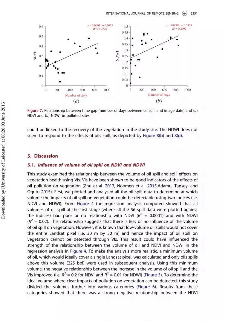
The relationship between the number of days and the VIs for all of the sites with oilspill greater than 225 bbl is presented in Figure 7. This figure shows that as the numberof days increases, so do the values of the VIs. This implies that with time, vegetationseems to recover from the effects of oil pollution. However, further analysis wasperformed by splitting the length of time into categories (0–1 year) and (1–2) year todetermine whether initially the vegetation would get affected and then recover after aspecific time. Results from this analysis are presented in Figure 8.
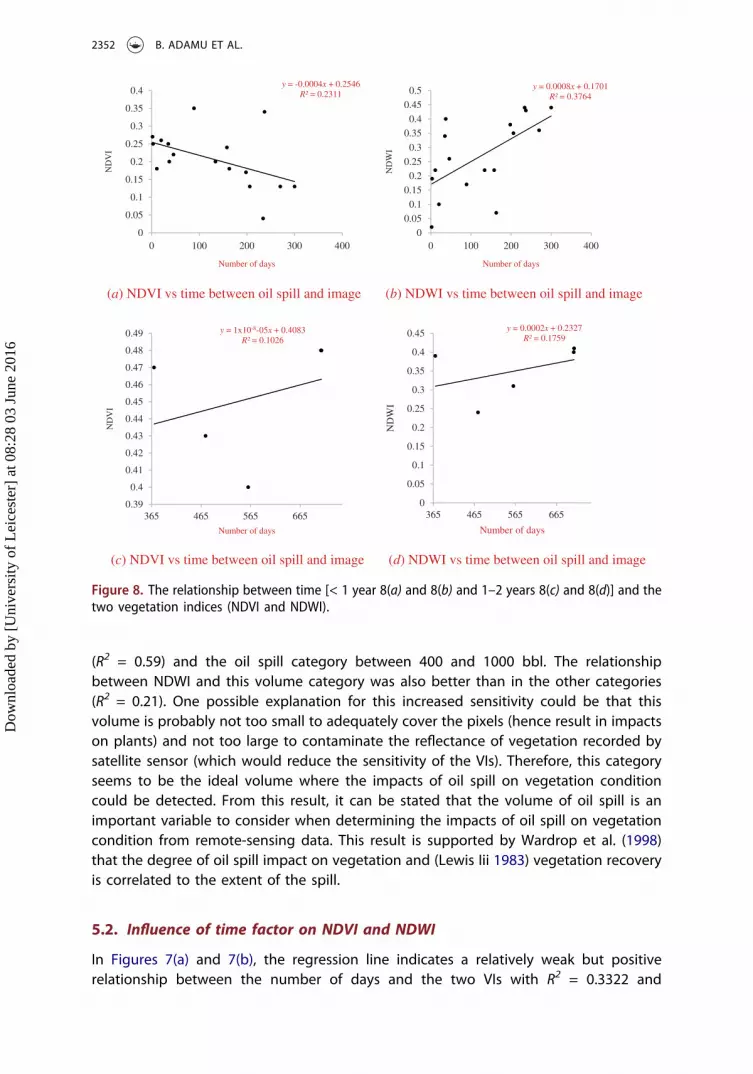
Figure 8(a) shows that the NDVI decreased in the first year, which could be attributedto the effects of oil spill, and started to increase in the second year (Figure 8(c), which
Table 3. Time gap between oil spill and image dates and NDVI and NDWIfor 25 spill sites with volume of oil spill volumes of more than > 225 bbl.Sample Points Oil Spill Volume (bbl) Time Gap (Days) NDVI NDWI
could be linked to the recovery of the vegetation in the study site. The NDWI does notseem to respond to the effects of oils spill, as depicted by Figure 8(b) and 8(d).
5. Discussion
5.1. Influence of volume of oil spill on NDVI and NDWI
This study examined the relationship between the volume of oil spill and spill effects onvegetation health using VIs. VIs have been shown to be good indicators of the effects ofoil pollution on vegetation (Zhu et al. 2013, Noomen et al. 2015,Adamu, Tansey, andOgutu 2015). First, we plotted and analysed all the oil spill data to determine at whichvolume the impacts of oil spill on vegetation could be detectable using two indices (i.e.NDVI and NDWI). From Figure 4 the regression analysis computed showed that allvolumes of oil spill at the first stage (where all the 56 spill data were plotted againstthe indices) had poor or no relationship with NDVI (R2 = 0.0001) and with NDWI(R2 = 0.02). This relationship suggests that there is less or no influence of the volumeof oil spill on vegetation. However, it is known that low-volume oil spills would not coverthe entire Landsat pixel (i.e. 30 m by 30 m) and hence the impact of oil spill onvegetation cannot be detected through VIs. This result could have influenced thestrength of the relationship between the volume of oil and NDVI and NDWI in theregression analysis in Figure 4. To make the analysis more realistic, a minimum volumeof oil, which would ideally cover a single Landsat pixel, was calculated and only oils spillsabove this volume (225 bbl) were used in subsequent analysis. Using this minimumvolume, the negative relationship between the increase in the volume of oil spill and theVIs improved (i.e. R2 = 0.2 for NDVI and R2 = 0.01 for NDWI) (Figure 5). To determine theideal volume where clear impacts of pollution on vegetation can be detected, this studydivided the volumes further into various categories (Figure 6). Results from thesecategories showed that there was a strong negative relationship between the NDVI
(a) (b)
y = 0.0003x + 0.2073R² = 0.3322
0
0.1
0.2
0.3
0.4
0.5
0.6
ND
VI
Number of days
y = 0.0002x + 0.2329R² = 0.2492
0
0.05
0.1
0.15
0.2
0.25
0.3
0.35
0.4
0.45
0.5
0 200 400 600 800 1000 0 200 400 600 800 1000
ND
WI
Number of days
Figure 7. Relationship between time gap (number of days between oil spill and image date) and (a)NDVI and (b) NDWI in polluted sites.
INTERNATIONAL JOURNAL OF REMOTE SENSING 2351
Dow
nloa
ded
by [
Uni
vers
ity o
f L
eice
ster
] at
08:
28 0
3 Ju
ne 2
016
(R2 = 0.59) and the oil spill category between 400 and 1000 bbl. The relationshipbetween NDWI and this volume category was also better than in the other categories(R2 = 0.21). One possible explanation for this increased sensitivity could be that thisvolume is probably not too small to adequately cover the pixels (hence result in impactson plants) and not too large to contaminate the reflectance of vegetation recorded bysatellite sensor (which would reduce the sensitivity of the VIs). Therefore, this categoryseems to be the ideal volume where the impacts of oil spill on vegetation conditioncould be detected. From this result, it can be stated that the volume of oil spill is animportant variable to consider when determining the impacts of oil spill on vegetationcondition from remote-sensing data. This result is supported by Wardrop et al. (1998)that the degree of oil spill impact on vegetation and (Lewis Iii 1983) vegetation recoveryis correlated to the extent of the spill.
5.2. Influence of time factor on NDVI and NDWI
In Figures 7(a) and 7(b), the regression line indicates a relatively weak but positiverelationship between the number of days and the two VIs with R2 = 0.3322 and
(a) NDVI vs time between oil spill and image (b) NDWI vs time between oil spill and image
(c) NDVI vs time between oil spill and image (d) NDWI vs time between oil spill and image
y = -0.0004x + 0.2546R² = 0.2311
0
0.05
0.1
0.15
0.2
0.25
0.3
0.35
0.4
ND
VI
Number of days
y = 0.0008x + 0.1701R² = 0.3764
0
0.05
0.1
0.15
0.2
0.25
0.3
0.35
0.4
0.45
0.5
ND
WI
Number of days
y = 1x10⁻⁸-05x + 0.4083R² = 0.1026
0.39
0.4
0.41
0.42
0.43
0.44
0.45
0.46
0.47
0.48
0.49
ND
VI
Number of days
y = 0.0002x + 0.2327R² = 0.1759
0
0.05
0.1
0.15
0.2
0.25
0.3
0.35
0.4
0.45
0 100 200 300 400 0 100 200 300 400
365 465 565 665 365 465 565 665
ND
WI
Number of days
Figure 8. The relationship between time [< 1 year 8(a) and 8(b) and 1–2 years 8(c) and 8(d)] and thetwo vegetation indices (NDVI and NDWI).
2352 B. ADAMU ET AL.
Dow
nloa
ded
by [
Uni
vers
ity o
f L
eice
ster
] at
08:
28 0
3 Ju
ne 2
016
R2 = 0.2224 for both NDVI and NDWI, respectively. This suggests that the time of imageacquisition can be a factor that influences the detectability of impacts of oil spills onvegetation. The VI values increase with increasing time between the image acquisitionand oil spill date, implying some form of vegetation recovery with time. To obtain a clearpicture of the impacts of time on the detectability of impacts of oil spill on vegetation,the data was divided into two categories (i.e. 0–1 year and 1–2 years) (Figure 8). Resultsfrom the NDVI showed that in the first year, there was a general decrease in its values(Figure 8(a)), implying the impacts of oil pollution on vegetation. After the first year, theNDVI values started to increase (Figure 8(c)), which implies that the impacted vegetationstarted to recover. The NDWI results did not show a similar pattern. Other researchershave shown that the impact of oil spills on vegetation can start to show within the firsttwo weeks of a spill event, and these can range from chlorosis to defoliation to treedeath (Duke and Burns 1999). However, these impacts can vary depending on thevegetation type, persistence of the oil spill (level of degradability), and the physicalfactors in the affected area (Hoff et al. 2002). A study in a mangrove reported that theamount of oil reaching the mangroves and the length of time spilled oil remains nearthe mangroves are key variables in determining the severity of effect (Garrity, Levings,and Burns 1993; Burns et al. 2002). The results from the NDVI in the current studyshowed that the impacts of oil spill on the mangrove forests were visible within the firstyear and the forests started to recover after the first year. Thus, it can be stated that thetime of image acquisition is an important factor to consider when studying the impactsof oil spills on vegetation using remote-sensing data.
6. Conclusion
The aim of this study was to test the influence of volume of oil spill and time gapbetween the image acquisition dates on the detectability of changes in vegetationstatus using VIs. First, all oil spills were used to test the influence of volume on thedetectability of pollution on vegetation condition using two VIs (i.e. NDVI and NDWI).Results from this showed a weak negative relationship between an increase in volumeand impacts on vegetation condition (i.e. reduction in NDVI and NDWI values). Aminimum volume (225 bbl), which was considered adequate to cover a single Landsatpixel, was calculated and used in subsequent analysis. The use of this minimumvolume improved the relationship between the VIs and oil spill volume. Furtheranalysis showed that the oil spill volume between 400 bbl and 1000 bbl resulted inthe most detectable influence of pollution on vegetation as shown by the strongnegative relationships between the VIs (especially NDVI) and this volume category.The analysis on the influence of time on the detectability of impacts of oil pollutionon vegetation showed that, in general, the longer the time between image acquisi-tion and oil spill, the lower the detectability of the impacts of pollution on thevegetation (showed by the positive relationship between NDVI/NDWI and time).However, further analysis showed that the NDVI was able to detect the effects onvegetation condition (indicated by the reduction in NDVI values) within the first yearof oil spill. In addition, the NDVI showed that the vegetation began to recover(increase in NDVI values) after the first year. Overall, as time increased between thedate of oil spill and image acquisition, the chances of detecting the impacts of oil
INTERNATIONAL JOURNAL OF REMOTE SENSING 2353
Dow
nloa
ded
by [
Uni
vers
ity o
f L
eice
ster
] at
08:
28 0
3 Ju
ne 2
016
pollution on vegetation seem to diminish. However, it is worth noting that theserelationships can be influenced by other factors such as the vegetation type, physicalcondition in the area, sensor characteristics, and type and persistence (degradability)of the oil (Pezeshki et al. 2000, Mendelssohn et al. 2012). The sensitivity of the indiceshas also contributed in the detection of oil spill. In conclusion, this study showed thatboth the volume of oil spill, and the time between image acquisition and spill dateare important factors to consider when using multispectral data to study the impactsof oil pollution on vegetation.
Disclosure statement
No potential conflict of interest was reported by the authors.
Funding
This work was supported and funded by the Petroleum Technology Development Fund (PTDF)under the Federal Government of Nigeria [PTDF/E/OSS/PHD/AB/347/11] and Modibbo AdamaUniversity of Technology, Yola, Nigeria.
References
Abbas, I. I. 2012. “An Assessment of Land Use/Land Cover Changes in a Section of Niger Delta,Nigeria.” Frontiers in Science 2: 137–143. doi:10.5923/j.fs.20120206.02.
Adamu, B., K. Tansey, and B. Ogutu. 2015. “Using Vegetation Spectral Indices to Detect OilPollution in the Niger Delta.” Remote Sensing Letters 6: 145–154. doi:10.1080/2150704X.2015.1015656.
Adejuwon, J. O. 2012. “Rainfall seasonality in the Niger Delta Belt, Nigeria.” Journal of Geographyand Regional Planning 5: 51–60.
Ajao, E., E. Oyewo, and J. Unyimadu. 1996. A Review of the Pollution of Coastal Waters in Nigeria.Lagos: Nigerian Institute for Oceanography and Marine Research.
Allen, J. R. L. 1965. “Late Quaternary Niger Delta, and Adjacent Areas: Sedimentary Environmentsand Lithofacies.” AAPG Bulletin 49: 547–600.
Arellano, P., K. Tansey, H. Balzter, and D. S. Boyd. 2015. “Detecting the Effects of HydrocarbonPollution in the Amazon Forest Using Hyperspectral Satellite Images.” Environmental Pollution205: 225–239. doi:10.1016/j.envpol.2015.05.041.
Avbovbo, A. A. 1978. “Tertiary Lithostratigraphy of Niger Delta: GEOLOGIC NOTES.” AAPG Bulletin62: 295–300.
BP. 2011. The BP Statistical Report of World Energy Report 2011. BP. Accessed 22 April 2014. http://www.bp.com/statisticalreview
Brekke, C., and A. H. S. Solberg. 2005. “Oil Spill Detection by Satellite Remote Sensing.” RemoteSensing of Environment 95: 1–13. doi:10.1016/j.rse.2004.11.015.
Bridge, G. 2008. “Global Production Networks and the Extractive Sector.” Governing Resource-BasedDevelopment Journal of Economic Geography 8: 387–419.
Brown, C. E., and M. F. Fingas. 2003. “Review of the Development of Laser Fluorosensors for OilSpill Application.” Marine Pollution Bulletin 47: 477–484. doi:10.1016/S0025-326X(03)00213-3.
Burke, K., T. Dessauvagie, and A. Whiteman. 1971. “Opening of the Gulf of Guinea and GeologicalHistory of the Benue Depression and Niger Delta.” Nature 233: 51–55.
Burns, G., R. Pond, P. Tebeau, and D. S. Etkin. 2002. “Looking to the Future––Setting the Agenda forOil Spill Prevention, Preparedness and Response in the 21st Century.” Spill Science & TechnologyBulletin 7: 31–37. doi:10.1016/S1353-2561(02)00057-9.
Casciello, D., T. Lacava, N. Pergola, and V. Tramutoli. 2007. “Robust Satellite Techniques (RST) for OilSpill Detection and Monitoring.” In International Workshop on the Analysis of Multi-TemporalRemote Sensing Images, 1–6. Leuven, July 18–20. Multitemp 2007. IEEE. doi:10.1109/MULTITEMP.2007.4293040.
Chander, G., B. L. Markham, and D. L. Helder. 2009. “Summary of Current Radiometric CalibrationCoefficients for Landsat MSS, TM, ETM+, and EO-1 ALI Sensors.” Remote Sensing of Environment113: 893–903. doi:10.1016/j.rse.2009.01.007.
CIA. 2005. World Fact Book [Online]. Accessed 21 October 2015. https://www.cia.gov/news-information/press-releases-statements/press-release-archive-2005/pr04282005.html
Duke, N. C., and K. A. Burns. 1999. Fate and Effects of Oil and Dispersed Oil on Mangrove Ecosystemsin Australia. Cape Cleveland: Australian Institute of Marine Science.
Duke, N. C., K. A. Burns, R. P. J. Swannell, O. Dalhaus, and R. J. Rupp. 2000. “Dispersant Use and aBioremediation Strategy as Alternate Means of Reducing Impacts of Large Oil Spills onMangroves: The Gladstone Field Trials.” Marine Pollution Bulletin 41: 403–412. doi:10.1016/S0025-326X(00)00133-8.
Fagbami, A. A., E. J. Udo, and C. T. I. Odu. 1988. “Vegetation Damage in an Oil Field in the NigerDelta of Nigeria.” Journal of Tropical Ecology 4: 61–75. doi:10.1017/S0266467400002510.
Gao, B.-C. 1996. “NDWI—A Normalized Difference Water Index for Remote Sensing of VegetationLiquid Water from Space.” Remote Sensing of Environment 58: 257–266. doi:10.1016/S0034-4257(96)00067-3.
Garrity, S. D., S. C. Levings, and K. A. Burns. 1993. “Chronic Oiling and Long-Term Effects of the1986 Galeta Spill on Fringing Mangroves.” International Oil Spill Conference Proceedings 1993 (1):319–324.
Goodman, R. 1994. “Overview and Future Trends in Oil Spill Remote Sensing.” Spill Science &Technology Bulletin 1: 11–21. doi:10.1016/1353-2561(94)90004-3.
Grimaz, S., S. Allen, J. Stewart, and G. Dolcetti. 2008. “Fast Prediction of the Evolution of OilPenetration into the Soil Immediately after an Accidental Spillage for Rapid-ResponsePurposes.” Proceeding of 3rd International Conference on Safety & Environment in ProcessIndustry, CISAP–3, Rome (I), May 11–14, Chemical Engineering Transactions, 2008. Citeseer.
Guyot, G., F. Baret, and S. Jacquemoud. 1992. “Imaging Spectroscopy for Vegetation Indices.”Imaging Spectroscopy: Fundamentals and Prospective Applications 2: 145–165.
Hoff, R., P. Hensel, E. Proffitt, P. Delgado, G. Shigenaka, R. Yender, and A. Mearns. 2002. Oil Spills inmangroves. Planning & Response Considerations. Darby, PA: National Oceanic and AtmosphericAdministration (NOAA). EUA. Technical Report.
IEA. 2011. World Energy Outlook. Accessed 22 April 2014. http://www.iea.org/publications/freepublications/…/WEO2011_WEB.pdf
Jha, M. N., J. Levy, and Y. Gao. 2008. “Advances in Remote Sensing for Oil Spill DisasterManagement: State-Of-The-Art Sensors Technology for Oil Spill Surveillance.” Sensors 8: 236–255. doi:10.3390/s8010236.
Landgrebe, D. A. 2005. Signal Theory Methods in Multispectral Remote Sensing. Hoboken, NJ: JohnWiley & Sons.
Lehr, W. J. 2001. “Review of Modeling Procedures for Oil Spill Weathering Behavior.” Advances inEcological Sciences 9: 51–90.
Lewis Iii, R. R. 1983. “Impact of Oil Spills on Mangrove Forests.” In Biology and Ecology ofMangroves. Dorchecht: Springer.
Mackay, D., and R. S. Matsugu. 1973. “Evaporation Rates of Liquid Hydrocarbon Spills on Land andWater.” The Canadian Journal of Chemical Engineering 51: 434–439. doi:10.1002/cjce.v51:4.
Mackay, D. A., and M. Mohtadi. 1975. “The Area Affected by Oil Spills on Land.” The CanadianJournal of Chemical Engineering 53: 140–143. doi:10.1002/cjce.v53:1.
Mendelssohn, I. A., G. A. Andersen, D. M. Baltz, R. H. Caffey, K. R. Carman, J. W. Fleeger, S. B. Joye, Q.Lin, E. Maltby, E. B. Overton, and L. P. Rozas. 2012. “Oil Impacts on Coastal Wetlands:Implications for the Mississippi River Delta Ecosystem after theDeepwater HorizonOil Spill.”BioScience 62: 562–574. doi:10.1525/bio.2012.62.6.7.
Myneni, R. B., S. Hoffman, Y. Knyazikhin, J. L. Privette, J. Glassy, Y. Tian, Y. Wang, X. Song, Y. Zhang,G. R. Smith, A. Lotsch, M. Friedl, J. T. Morisette, P. Votava, R. R. Nemani, and S. W. Running. 2002.“Global Products of Vegetation Leaf Area and Fraction Absorbed PAR from Year One of MODISData.” Remote Sensing of Environment 83: 214–231. doi:10.1016/S0034-4257(02)00074-3.
Noomen, M. F., A. Hakkarainen, M. van der Meijde, and H. M. A. van der Werff. 2015. “Evaluatingthe Feasibility of Multitemporal Hyperspectral Remote Sensing for Monitoring Bioremediation.”International Journal of Applied Earth Observation and Geoinformation 34: 217–225. doi:10.1016/j.jag.2014.08.016.
Noomen, M. F., K. L. Smith, J. J. Colls, M. D. Steven, A. K. Skidmore, and F. D. van der Meer. 2008.“Hyperspectral Indices for Detecting Changes in Canopy Reflectance as a Result of UndergroundNatural Gas Leakage.” International Journal of Remote Sensing 29: 5987–6008. doi:10.1080/01431160801961383.
Noomen, M. F., H.M.A van der Werff, and F. D. van der Meer. 2012. “Spectral and Spatial Indicatorsof Botanical Changes Caused by Log-Term Hydrocarbon Seepage.” Ecological Informatics 5: 55–64. doi:10.1016/j.ecoinf.2012.01.001.
Obire, O., and O. Nwaubeta. 2002. “Effects of Refined Petroleum Hydrocarbon on SoilPhysiochemical and Bacteriological Characteristics.” Journal of Applied Science Environment 6:39–44.
Oguntunde, P. G., B. J. Abiodun, and G. Lischeid. 2011. “Rainfall Trends in Nigeria, 1901–2000.”Journal of Hydrology 411: 207–218. doi:10.1016/j.jhydrol.2011.09.037.
Oliveira, W. J. D., A. P. Crosta, and J. L. M. Goncalves. 1997. “Spectral Characteristics of Soils andVegetation Affected by Hydrocarbon Gas: A Greenhouse Simulation of the Remanso Do FogoSeepage.” Paper presented at the Twelfth International and Workshops on Applied geologicremote Sensing, Denver, CO.
Pezeshki, S. R., M. W. Hester, Q. Lin, and J. A. Nyman. 2000. “The Effects of Oil Spill and Clean-Up onDominant US Gulf Coast Marsh Macrophytes: A Review.” Environmental Pollution 108: 129–139.doi:10.1016/S0269-7491(99)00244-4.
Purkis, S., and V. Klemas. 2011. Remote Sensing and Global Environmental Change. West Sussex UK:Wiley-Blackwell & Sons Ltd.
Reed, M., Ø. Johansen, P. J. Brandvik, P. Daling, A. Lewis, R. Fiocco, D. Mackay, and R. Prentki. 1999.“Oil Spill Modeling towards the Close of the 20th Century: Overview of the State of the Art.” SpillScience & Technology Bulletin 5: 3–16. doi:10.1016/S1353-2561(98)00029-2.
Serra-Sogas, N., P. D. O’hara, R. Canessa, P. Keller, and R. Pelot. 2008. “Visualization of SpatialPatterns and Temporal Trends for Aerial Surveillance of Illegal Oil Discharges in WesternCanadian Marine Waters.” Marine Pollution Bulletin 56: 825–833. doi:10.1016/j.marpolbul.2008.02.005.
Short, J. 2003. “Long-Term Effects of Crude Oil on Developing Fish: Lessons from the Exxon ValdezOil Spill.” Energy Sources 25: 509–517. doi:10.1080/00908310390195589.
Short, K., and A. Stauble. 1967. “Outline of Geology of Niger Delta.” AAPG Bulletin 51: 761–779.Simmons, C. S., J. M. Keller, and J. L. Hylden. 2004. Spills on Flat Inclined Pavements. Washington,
DC: Department of Energy.Simmons, C. S. A., and J. M. Keller. 2003. Status of Models for Land Surface Spills of Nonaqueous
Liquids. Washington, DC: Pacific Northwest National Laboratory.Sims, D. A. 2002. “Relationship between Leaf Pigment Content and Spectral Reflectance across a
Wide Range of Species, Leaf Structures and Developmental Stages.” Remote Sensing ofEnvironment 18: 337–354. doi:10.1016/S0034-4257(02)00010-X.
Slonecker, T., G. B. Fisher, D. P. Aiello, and B. Haack. 2010. “Visible and Infrared Remote Imaging ofHazardous Waste: A Review.” Remote Sensing 2: 2474–2508. doi:10.3390/rs2112474.
Smil, V. 2010. Energy Transitions: History, Requirements, Prospects. Oxford, England: Praeger AnImprint of ABC-CLIO, LLC.
UNEP. 2011. Environmental Assessment of Ogoniland. Nairobi: United Nations EnvironmentalProgramme.
van der Meer, F., P. Van Dijk, H. van der Werff, and H. Yang. 2002. “Remote Sensing and PetroleumSeepage: A Review and Case Study.” Terra Nova 14: 1–17. doi:10.1046/j.1365-3121.2002.00390.x.
van der Werff, H., M. van der Meijde, F. Jansma, F. van der Meer, and G. J. Groothuis. 2008. “ASpatial-Spectral Approach for Visualization of Vegetation Stress Resulting from PipelineLeakage.” Sensors 8: 3733–3743. doi:10.3390/s8063733.
Wardrop, J., B. Wagstaff, P. Pfennig, J. Leeder, and R. Connolly. 1998. The Distribution, Persistenceand Effects of Petroleum Hydrocarbons in Mangroves Impacted by the ‘Era Oil Spill’(September1992). Adelaide: Office of the Environment Protection Authority, South Australian Department ofEnvironment and Natural Resources.
Yim, U. H., S. Y. Ha, J. G. An, J. H. Won, G. M. Han, S. H. Hong, M. Kim, J.-H. Jung, and W. J. Shim.2011. “Fingerprint and Weathering Characteristics of Stranded Oils after the Hebei Spirit OilSpill.” Journal of Hazardous Materials 197: 60–69. doi:10.1016/j.jhazmat.2011.09.055.
Zhao, Q., and Y. Li. 2007. “Monitoring Marine Oil-spill Using Microwave Remote SensingTechnology. Electronic Measurement and Instruments, 2007.” ICEMI ‘07. 8th InternationalConference on, August 16 2007-July 18 2007.4–69-4–72.
Zhu, L., X. Zhao, L. Lai, J. Wang, L. Jiang, J. Ding, N. Liu, et al. 2013. “Soil TPH ConcentrationEstimation Using Vegetation Indices in an Oil Polluted Area of Eastern China.” PLoS One 8:e54028. doi:10.1371/journal.pone.0054028.