2011 INTERNATIONAL OIL SPILL CONFERENCE

1 2011-428

Tracking and Modeling the Degradation of a 30 Year Old Fuel Oil Spill with

Comprehensive Two-Dimensional Gas Chromatography

March 14, 2011

Glenn S. Frysinger1, Gregory J. Hall

1, Ariana L. Pourmonir

1, Heather N. Bischel

2, Emily E.

Peacock2, Robert N. Nelson

2, Christopher M. Reddy

2

1Department of Science, U.S. Coast Guard Academy, 27 Mohegan Ave. New London, CT 06320

2Department of Marine Chemistry & Geochemistry, Woods Hole Oceanographic Institution, 266

Woods Hole Rd. Woods Hole, MA. 02543

ABSTRACT

On October 9, 1974, the barge Bouchard 65, carrying 12 million liters of No. 2 fuel oil,

spilled an undetermined amount of oil off the west entrance of the Cape Cod Canal in Buzzards

Bay, Massachusetts, USA. Wind patterns and currents caused significant oiling of the nearby

Winsor Cove salt marsh. Fortunately, an original Bouchard 65 cargo oil sample was retained

from the spill which offers a unique opportunity to compare in vitro weathering experiments with

petroleum that has been weathered naturally for over thirty years. Samples of the original

product were bio-weathered in the lab over a period of days, and then these samples, plus a

contemporary sample from Winsor Cove, were analyzed by Comprehensive two-dimensional gas

chromatography with Time of Flight Mass Spectrometry detection (GC×GC-MS). The data

from the laboratory experiment was used to create a Principal Components Regression model to

predict amount of weathering. The environmental sample was projected onto the regression

model and fit most well at approximately 13 days of laboratory weathering time. Examination of

the regression vector from PCR shows mass ions related to polar and volatile compounds

decreased first, while mass ions and peaks related to sesquiterpanes persisted during the

weathering process.

INTRODUCTION

On October 9, 1974, the barge Bouchard 65, carrying 12 million liters of No. 2 fuel oil,

spilled an undetermined amount of oil off the west entrance of the Cape Cod Canal in Buzzards

Bay, Massachusetts, USA. Wind patterns and currents caused significant oiling of the nearby

Winsor Cove salt marsh, (Hampson and Moul, 1978). Studies conducted in the first three years

after the spill found that oil persisted in the marsh, but some oil components such as alkyl

substituted PAHs had decreased (Teal et al., 1978). Sediment cores collected between 2001 and

2005, 30 years after the spill, showed that heavily weathered and degraded oil was still

detectable in the upper 4 cm of the marsh sediment. Total petroleum hydrocarbons (TPHs) were

found to be 8.7 mg g-1

(dry weight) and polycyclic aromatic hydrocarbons (PAHs) were 16.7 μg

g-1

for total alkyl-substituted naphthalenes and phenanthrenes (Peacock et al., 2007).

Fortunately, an original Bouchard 65 cargo oil sample was retained from the 1974 spill so

comparisons can be made between the chemical composition of the original oil and the degraded

oil remaining in the Winsor Cove sediments after 30 years. In laboratory experiments, the

Bouchard 65 No. 2 fuel oil was biodegraded under aerobic, nutrient-rich conditions in order to

2011 INTERNATIONAL OIL SPILL CONFERENCE

2 2011-428

simulate the biodegradation that occurred at Winsor Cove. A degradation model can be

constructed from the laboratory experiments to calibrate the extent of natural weathering of

petroleum compounds in Winsor Cove sediments.

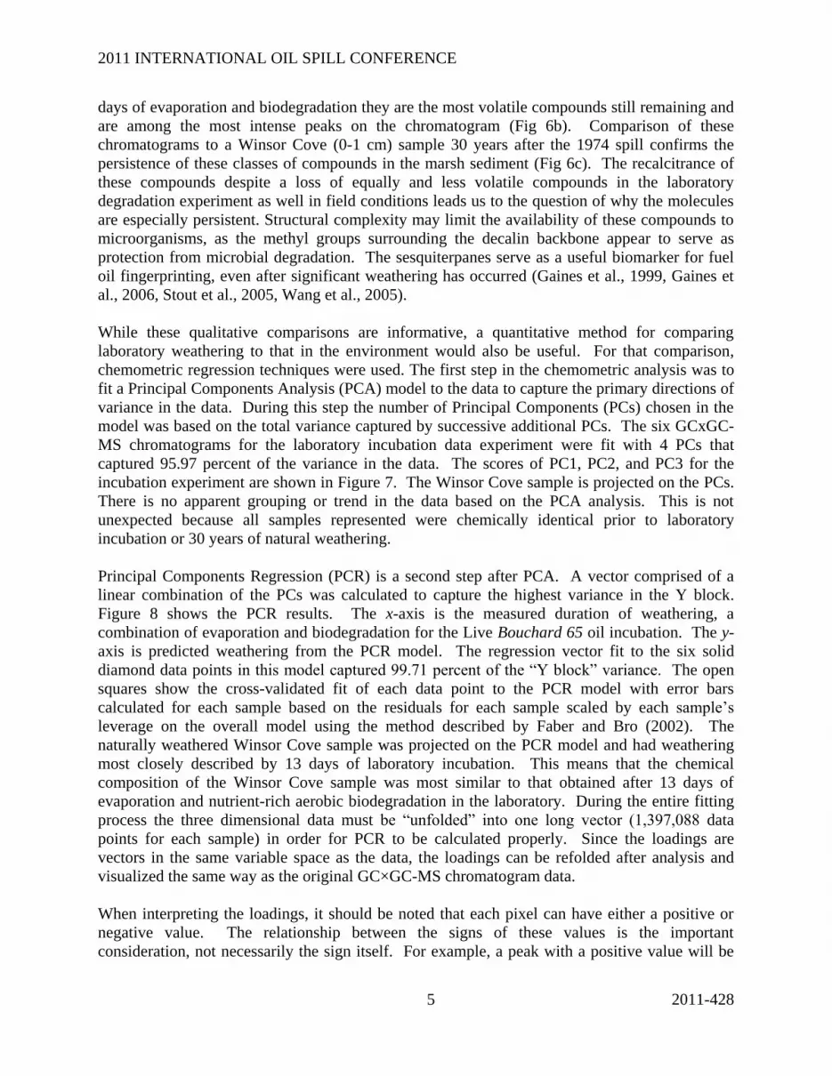
Comprehensive two-dimensional gas chromatography (GC×GC) produces a high resolution

separation in order to identify and quantify individual compounds in complex samples like

petroleum. GC×GC is a two column gas chromatography method where the first column is

typically nonpolar for a volatility-based separation, and the second column is polar for a polarity-

based separation. Coeluting analytes from the first column are periodically trapped and

concentrated with a modulator and then injected (3 s cycle time) into the second column for a

rapid separation via a different retention mechanism. While single column GC can resolve 100s

of peaks, GC×GG separations have a peak capacity that is a product of the two columns so 1000s

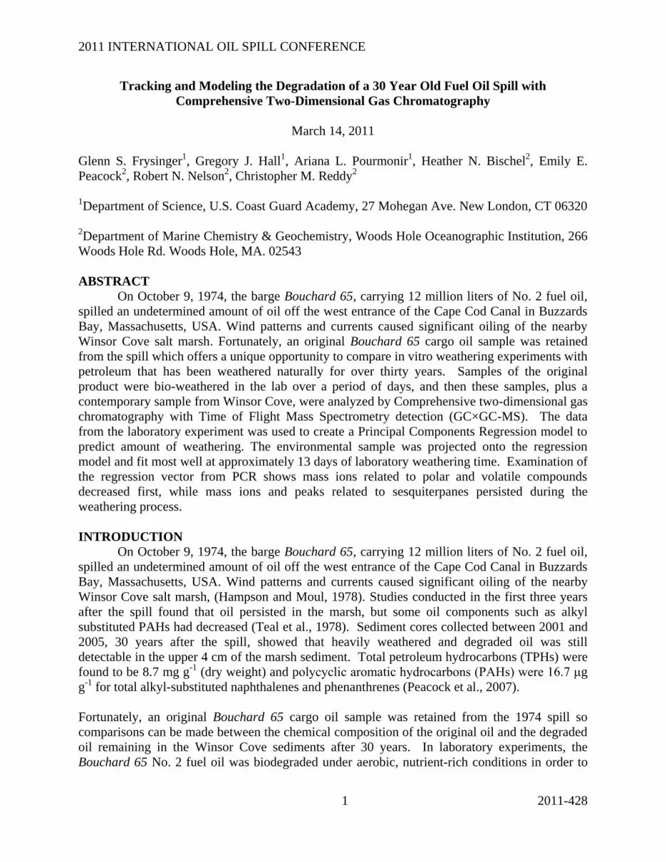
of peaks are routinely resolved. A GC and GC×GC-MS total ion chromatogram of a fuel oil is

shown in Figure 1. The x-axis shows a volatility based separation. The C9 to C21 n-alkanes are

seen ranging from left to right as large equally spaced peaks. The y-axis shows the rapid polarity

based separations that effectively resolve the first column coelutions. Peaks are reconstructed as

a color contour plot from the total ion signal of hundreds of second-column chromatograms. As

second-column retention time increases, the one-and two-ring cycloalkanes, and the one- two-

and three-ring aromatics are separated. Examination of each vertical slice shows that multiple

coeluters have been resolved. In addition to producing more separated peaks per time, GC×GC

is known for its ability to separate and group chemical compounds by class (Dimandja, 2004,

Gaines et al, 2007). If coupled to a time-of-flight mass spectrometer, there is a full scan mass

spectrum for each GC×GC separated peak. The mass spectra are interference free because

components are chromatographically separated prior to mass spectrum measurement.

The data density of GC×GC-MS chromatograms is high. A 90 minute chromatogram as shown

in Figure 1 will consist of 540,000 individual mass spectra (100 Hz, m/z 45-250) for more than

110 million data points per chromatogram. Chemometric approaches that use multivariate

statistical analyses are a proven method to analyze large data sets and produce an unbiased

determination of which chromatogram data describe the variance between multiple GC×GC-MS

chromatograms. Both principal component analysis (PCA) and principal component regression

(PCR) methods will be used to analyze the fuel oil biodegradation time series. PCA is a method

that reduces data dimensionality to identify a reduced number of orthogonal variables (PCs) that

describe the majority of the data variance. The results are displayed as two- or three-dimensional

scores plots that frequently show grouping of related samples. In addition to the scores, the

loadings identify which variables (such as which chromatogram peaks) contribute most to the

variance. In some cases, samples are not distinctly ordered in the PCA scores plot according to

the specific characteristic of interest, so regression (PCR) is required to determine the linear

combination of the PCs that captures the variance in the regression variable, which is typically

called the “Y block”. Many studies have been published using chemometric techniques for

fingerprinting or classification, only a few have focused on regression (Pierce et al., 2008;

Mispaleer et al., 2003).

The goals of the described experiments include:

1.) The use of GC×GC-MS analysis to describe the weathering loss of chemical

compounds from a fuel oil after 30 years of natural degradation.

2011 INTERNATIONAL OIL SPILL CONFERENCE

3 2011-428

2.) The completion of laboratory degradation experiments to simulate the biodegradation

of fuel oil for comparison to petroleum weathered in the environment.

3.) The application of PCA and PCR chemometric methods to assist these analyses and to

calibrate the rate of degradation in laboratory experiments.

METHODS

Incubations

Live and Control incubations of the Bouchard 65 No. 2 fuel oil cargo were prepared in 4-

L amber glass bottles with 200-300 g of 1 mm-sieved sediment (dry weight) and 700-1000 mL

autoclaved, 0.2 μm-filtered seawater. Oil-free sediment samples containing natural oil-degrading

microbes were collected from Wild Harbor Marsh site M-1. Nutrients as 0.25g NH4Cl and 0.2g

KH2PO4 were introduced to each incubation. The Control incubation was autoclaved (40 min/40

min exhaust) and spiked with 50 g azide dissolved in seawater (10g added initially, 40g added

after 2 weeks). Live and Control incubations were spiked with 1.2 g neat Bouchard 65 No. 2

fuel oil. The incubations were covered with foil to block out light, stirred for the duration of the

experiment, and kept under humidified air (approximate flow rate 180 mL min-1

). Duplicate

sediment samples were taken from each incubation at Day 0, 6, 11, 20, 36 and 46. One gram of

air-dried sediment was spiked with Hexatriacontane (n-C36, 15 μg) and extracted with

dichloromethane:methanol (9:1) by accelerated solvent extraction (100 C, 1000 psi). Extracts

were concentrated by rotary evaporation and percolated through a sodium sulfate column eluted

with dichloromethane to remove water. Extracts were reduced in volume (≤ 1mL).

GC Analysis

The samples were analyzed on an Agilent 6890 series gas chromatograph with a Flame

Ionization Detector (FID). A 1 uL sample was injected splitless to a polydimethylsiloxane

capillary column (J&W DB-5MS, 60.0m, 0.32-mm I.D., 0.25-um film) with GC oven

temperature, 60°C (1 min), 20°C min-1

to 80°C (3 min), 5°C min-1

to 320°C (20 min). Helium

was the carrier gas at 1.5 ml min-1

constant flow. Total Petroleum Hydrocarbon (TPH)

quantification was determined with calibration solutions of n-C36, stearyl palmitate and

Bouchard 65 No. 2 fuel oil.

GC×GC-MS

The GCGC-MS system used to analyze the sediment extracts was a Leco Pegasus 4D

system consisting of an Agilent 6890 gas chromatograph configured with a split injector, two

chromatography columns, a liquid nitrogen-cooled pulsed jet modulator, and a unit mass

resolution time-of-flight mass spectrometer. A 1.0 μL sediment extract sample was injected into

a 250 C split injector with a 20:1 split ratio. The first-dimension separation was performed on a

nonpolar polydimethylsiloxane phase (Phenomenex, ZB-1, 30.0 m, 0.25 mm I.D., 1.0-μm film)

with GC oven temperature 40°C (1 min) , 3 C min-1

to 300 C. The modulation column was

deactivated column (1.0 m, 0.10 mm I.D.) with temperature 140°C (1 min), 3 C min-1

to 400

C. The second-dimension separation was performed on a polar 50% phenyl equivalent

polysiloxane phase (SGE, BPX-50, 3.5 m, 0.10 mm I.D., 0.1 μm film) with GC oven temperature

40°C (1 min), 3 C min-1

to 300 C. Hydrogen was the carrier gas at 1.2 mL min-1

constant

flow. The GC×GC modulator period was 3 s. The ToF detector collected spectra from m/z 45 to

250 at 100Hz.

2011 INTERNATIONAL OIL SPILL CONFERENCE

4 2011-428

Chemometrics

GC×GC-MS data was baseline corrected with CGImage, v2.1 and imported as comma

separated value (.csv) file to MATLAB v 2010b where it was compiled into a single dataset

object (DSO) with PLS_Toolbox®

v6.0.1 published by Eigenvector Research Inc. A smaller

region from 46.4 to 57.6 min range on the first dimension and 0.2 to 2.5 s on the second

dimension was selected for PCA and PCR analysis. The reduced range focused on a region of

the chromatogram with high peak density and significant changes caused by biodegradation. In

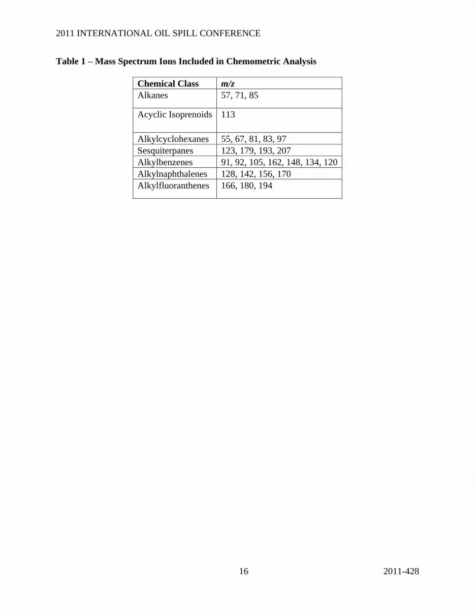
the mass spectra, only ions that represent specific petroleum classes and useful for oil

fingerprinting were included in the data set (ASTM, 2006; ASTM, 2010). The ions and

associated chemical classes are listed in Table 1. The final DSO contained seven GC×GC-MS

chromatograms with 224 points in the first dimension by 231 points in the second dimension by

27 selected mass ions. Prior to the fit of a chemometric model the data was pre-processed by

unit normalization to offer equal leverage to each sample, and then mean-centered to center the

data at the origin. The regression or “Y block” (predicted variable) was mean-centered to match.

RESULTS / DISCUSSION

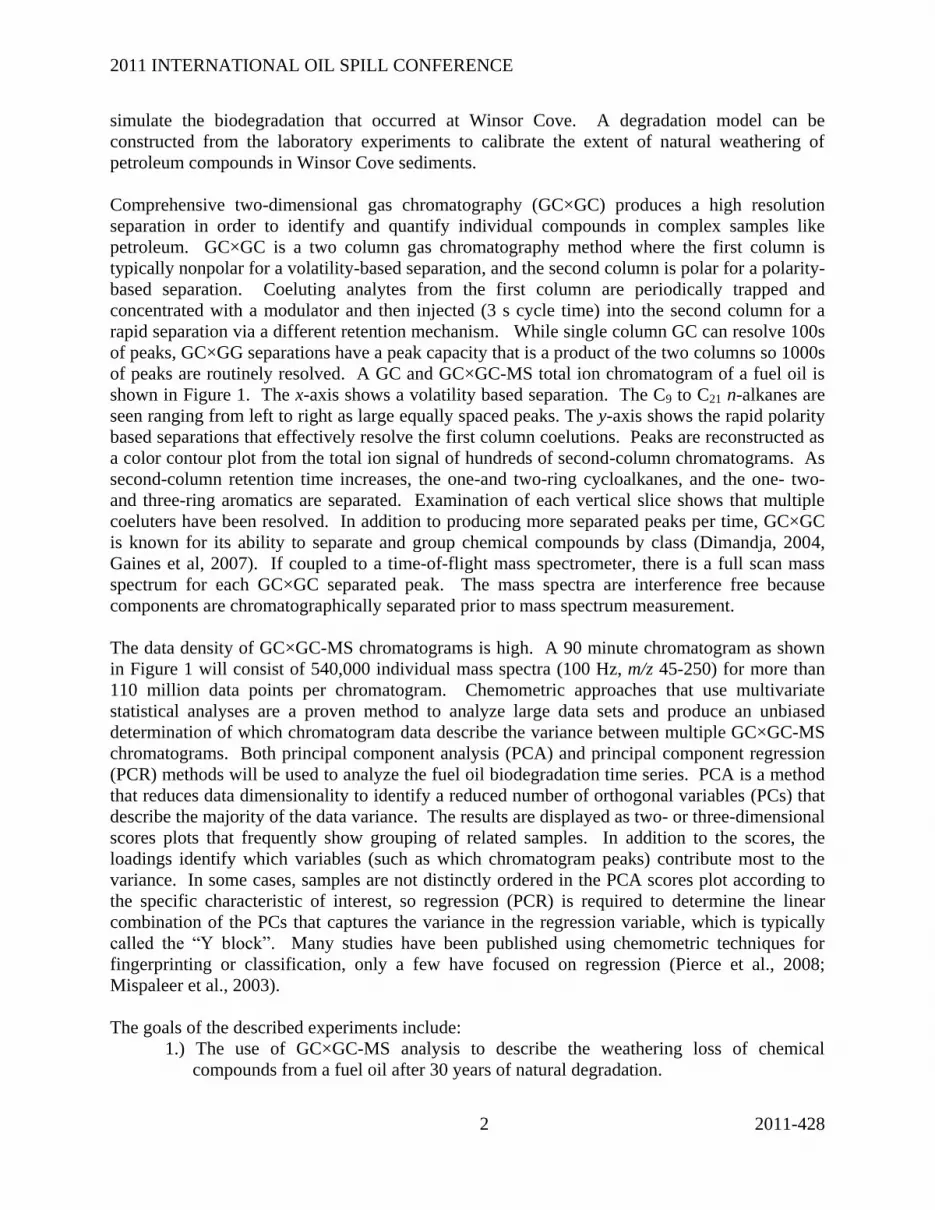
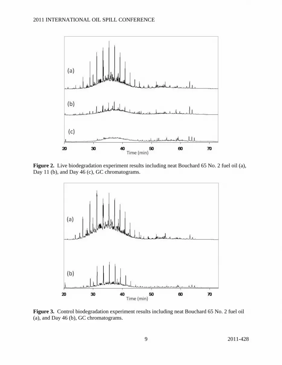
Figures 2a-c show the gas chromatograms for the Live incubation results for the

Bouchard 65 fuel oil sample at Day 0, 11 and 46 respectively. Prevalent n-alkane and branched

alkane peaks apparent in Day 0 are significantly smaller by Day 11 and nearly indiscernible by

Day 46 of the experiment. As the prominent n-alkanes are degraded, the chromatogram

transforms to an unresolved complex mixture (UCM) hump with few chromatographically

resolved peaks. Figures 3a-b for the Control incubation show persistence of the n-alkanes

throughout the 46 day incubation period. Comparison of the Live and Control experiment can be

used to determine the factors contributing to degradation. The Control experiment shows an

overall loss of fuel oil mass and a preferential loss of the more volatile, lower molecular weight

compounds. This weathering loss can be attributed to evaporation. The Live experiment with

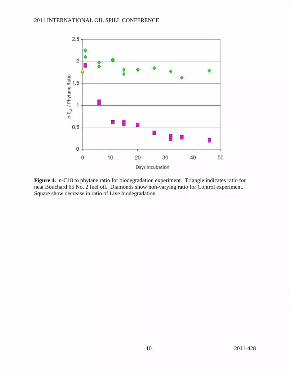
the loss of n-alkanes shows the additional contribution of microbial degradation. A plot of the n-

C18 to phytane peak ratios versus time in Figure 4 reveals a significant decrease in the ratio for

the Live incubation within the first 11 days of the experiment and a continued downward slope

through Day 46 suggesting strong microbe activity. Branched isoprenoid alkanes such as

phytane are generally more difficult for microorganisms to degrade than straight chain straight

chain alkanes, so a decrease of n-C18 relative to phytane is a classic indication of microbial

activity. The ratio remains relatively constant in the Control incubation, confirming the absence

of microorganisms.

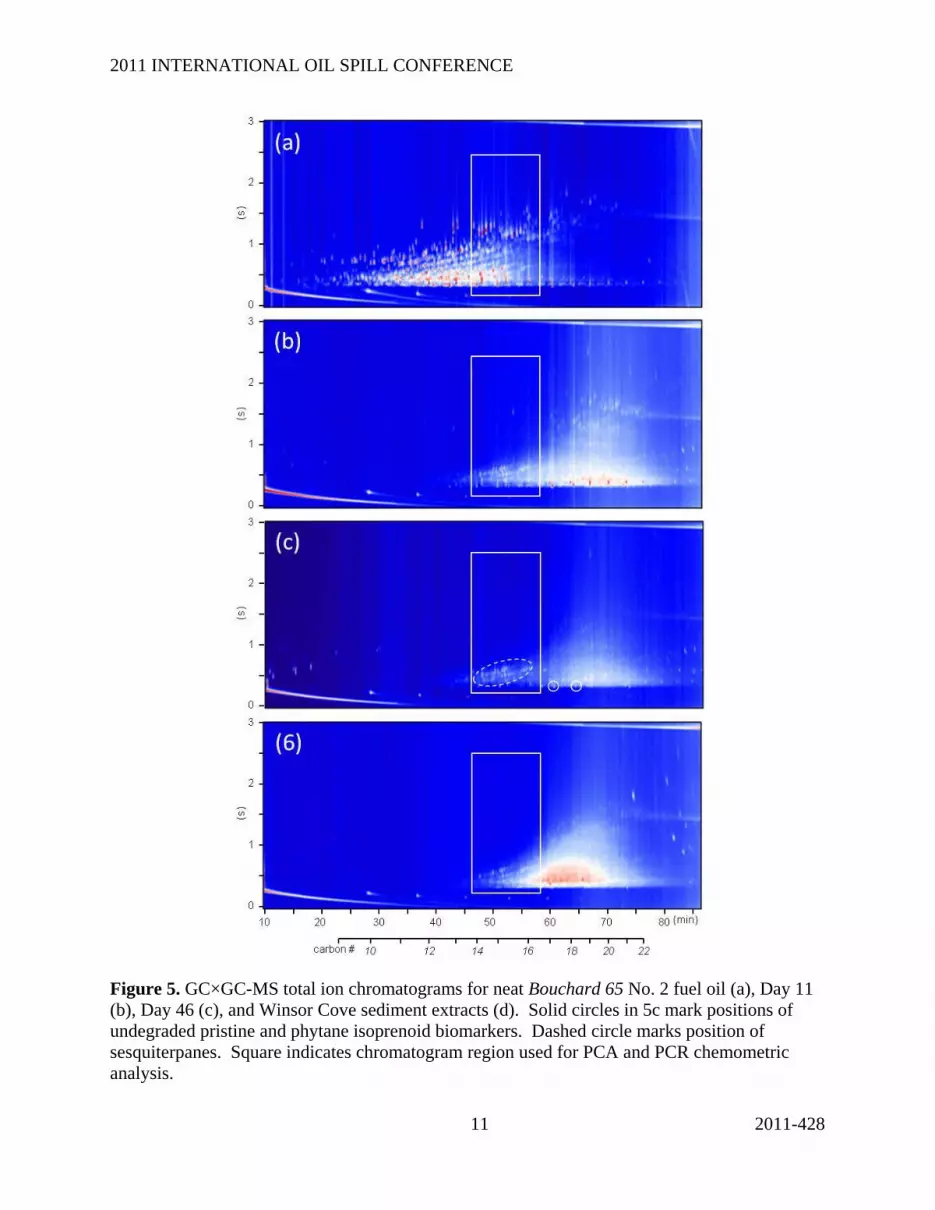
Two-dimensional GC×GC-MS total ion chromatograms are shown in Figures 5a-d. Panel 5a is

the Bouchard 65 cargo oil, panels 5b and 5c are the Day 11 and Day 46 Live incubations, and

panel 5d is the Winsor Cove (0-1 cm) sediment sample. Comparison of the Bouchard 65 cargo

oil with the Day 11 incubation shows that there is a near total loss of compounds smaller than n-

C15 and a complete loss of alkyl substituted benzenes, naphthalenes, and phenanthrenes across

the whole chromatogram. The Day 46 incubation shows even more significant weathering. The

most prominent peaks remaining are the pristane and phytane isoprenoids (marked with solid

circles) and a series of C5- and C6-subsituted decalins in the C15 – C16 retention index range

(marked with dashed circle). These compounds are commonly known as sesquiterpanes. This

chromatogram region is expanded in Figures 6a-c as m/z 123 extracted ion chromatograms. The

sesquiterpanes are not among the most abundant compounds in the fresh oil sample, but after 46

2011 INTERNATIONAL OIL SPILL CONFERENCE

5 2011-428

days of evaporation and biodegradation they are the most volatile compounds still remaining and

are among the most intense peaks on the chromatogram (Fig 6b). Comparison of these

chromatograms to a Winsor Cove (0-1 cm) sample 30 years after the 1974 spill confirms the

persistence of these classes of compounds in the marsh sediment (Fig 6c). The recalcitrance of

these compounds despite a loss of equally and less volatile compounds in the laboratory

degradation experiment as well in field conditions leads us to the question of why the molecules

are especially persistent. Structural complexity may limit the availability of these compounds to

microorganisms, as the methyl groups surrounding the decalin backbone appear to serve as

protection from microbial degradation. The sesquiterpanes serve as a useful biomarker for fuel

oil fingerprinting, even after significant weathering has occurred (Gaines et al., 1999, Gaines et

al., 2006, Stout et al., 2005, Wang et al., 2005).

While these qualitative comparisons are informative, a quantitative method for comparing

laboratory weathering to that in the environment would also be useful. For that comparison,

chemometric regression techniques were used. The first step in the chemometric analysis was to

fit a Principal Components Analysis (PCA) model to the data to capture the primary directions of

variance in the data. During this step the number of Principal Components (PCs) chosen in the

model was based on the total variance captured by successive additional PCs. The six GCxGC-

MS chromatograms for the laboratory incubation data experiment were fit with 4 PCs that

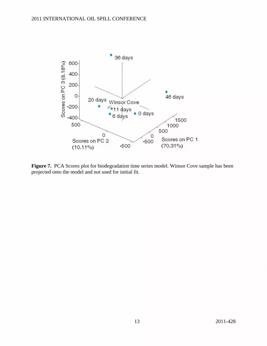
captured 95.97 percent of the variance in the data. The scores of PC1, PC2, and PC3 for the

incubation experiment are shown in Figure 7. The Winsor Cove sample is projected on the PCs.

There is no apparent grouping or trend in the data based on the PCA analysis. This is not

unexpected because all samples represented were chemically identical prior to laboratory

incubation or 30 years of natural weathering.

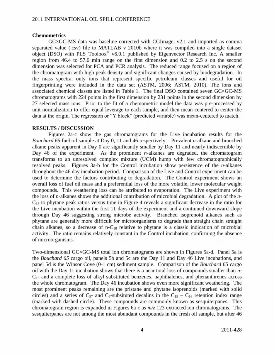
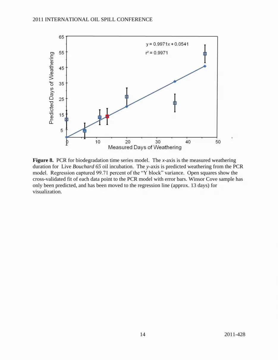
Principal Components Regression (PCR) is a second step after PCA. A vector comprised of a

linear combination of the PCs was calculated to capture the highest variance in the Y block.

Figure 8 shows the PCR results. The x-axis is the measured duration of weathering, a

combination of evaporation and biodegradation for the Live Bouchard 65 oil incubation. The y-

axis is predicted weathering from the PCR model. The regression vector fit to the six solid

diamond data points in this model captured 99.71 percent of the “Y block” variance. The open

squares show the cross-validated fit of each data point to the PCR model with error bars

calculated for each sample based on the residuals for each sample scaled by each sample’s

leverage on the overall model using the method described by Faber and Bro (2002). The

naturally weathered Winsor Cove sample was projected on the PCR model and had weathering

most closely described by 13 days of laboratory incubation. This means that the chemical

composition of the Winsor Cove sample was most similar to that obtained after 13 days of

evaporation and nutrient-rich aerobic biodegradation in the laboratory. During the entire fitting

process the three dimensional data must be “unfolded” into one long vector (1,397,088 data

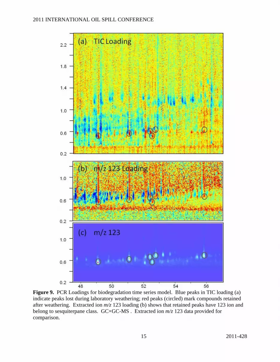
points for each sample) in order for PCR to be calculated properly. Since the loadings are

vectors in the same variable space as the data, the loadings can be refolded after analysis and

visualized the same way as the original GC×GC-MS chromatogram data.

When interpreting the loadings, it should be noted that each pixel can have either a positive or

negative value. The relationship between the signs of these values is the important

consideration, not necessarily the sign itself. For example, a peak with a positive value will be

2011 INTERNATIONAL OIL SPILL CONFERENCE

6 2011-428

changing opposite to the direction a peak with a negative value is changing. The effect of unit

normalization in this data is to make peaks that are unchanging with weathering seem positive

since they are becoming more important with respect to the total mass left in the sample.

Negative peaks are those compounds disappearing first as a result of the weathering. Figure 9a

shows the GCxGC-MS total ion (TIC) loadings. The blue peaks indicate peaks lost during the

laboratory fuel oil weathering, the red peaks mark compounds retained in the sample. The

predominance of blue peaks is expected because weathering was significant in the chromatogram

region used for the model (see Figures 5a-c). The few large red peaks observed in the TIC

loadings (Fig 9a) are also observed in the m/z 123 loadings (Fig 9b). This confirms that the

compound peaks identified as being degradation resistant using the PCR model were

sesquiterpanes. Figure 9c is the original GC×GC-MS m/z 123 data for the Day 46

biodegradation sample scaled equivalently for comparison.

Principal Components Regression of GC×GC-MS data has provided a quantitative calibration

between laboratory weathering experiments and naturally weathered oil. This method is more

informative than simple peak ratios, but also is consistent with the results obtained by those

ratios. The examination of regression vectors of these multivariate data sets can show important

chemical information that can be used for future investigations into both fingerprinting and

weathering extent.

REFERENCES

ASTM Standard D5739. 2006. " Standard practice for oil spill identification by gas

chromatography and positive ion electron impact low resolution mass spectrometry,” ASTM

International, West Conshohocken, PA, 2006.

ASTM Standard E1618. 2010. “Standard test method for ignitable liquid residues in extracts

from fire debris samples by gas chromatography-mass spectrometry,” ASTM International, West

Conshohocken, PA, 2010.

Dimandja, J-M.D. 2004. Comprehensive 2-D GC provides high-performance separations in

terms of selectivity, sensitivity, speed, and structure. Analytical Chemistry 76:167A–174A

Faber, N.M. and R. Bro. 2002. Standard error for multiway PLS: 1. Background and a simulation

study. Chemomem. and Intell. Syst. 61:133–149

Gaines, R.B., G.S. Frysinger, M.S. Hendrick-Smith, and J.D. Stuart. 1999. Oil spill identification

by comprehensive two-dimensional gas chromatography (GC×GC). Environmental Science

&Technology 33:2106–112.

Gaines, R.B., G.J. Hall, G.S. Frysinger, W.R. Gronlund, and K.L. Juaire. 2006. Chemometric

determination of target compounds used to fingerprint unweathered diesel fuels. Environmental

Forensics 7:1–12.

Gaines, R.B., G.S. Frysinger, C.M. Reddy, and R.K. Nelson. 2007. Oil spill identification by

comprehensive two-dimensional gas chromatography (GC × GC), Chapter 5, in Oil Spill

2011 INTERNATIONAL OIL SPILL CONFERENCE

7 2011-428

Environmental Forensics – Fingerprinting and Source Identification. Z. Wang, S.A. Stout Eds.

Elsevier.

Hampson, G.R., and E.T. Moul. 1978. No. 2. Fuel oil spill in Bourne, Massachusetts: immediate

assessment of the effects on marine invertebrates and a 3-year study of growth and recovery of a

salt marsh. Journal of the Fisheries Research Board of Canada 35:731–744.

Peacock, E.E., G.R. Hampson, R.K. Nelson, L. Xu, G.S. Frysinger, R.B. Gaines, J.W.

Farrington, B.W. Tripp, and C.M. Reddy. 2007. The 1974 spill of the Bouchard 65 oil barge:

Petroleum hydrocarbons persist in Winsor Cove salt marsh sediments. Marine Pollution Bulletin

54: 214–225

Pierce K.M., J.C. Hoggard, R.E. Mohler, and R.E. Synovec. 2008. Recent advancements

in comprehensive two-dimensional separations with chemometrics. Journal of Chromatography

A. 1184:341–52.

Stout, S.A., A.D. Uhler, and K.J McCarthy. 2005. Middle distillate fuel fingerprinting using

drimane-based bicyclic sesquiterpanes. Environmental Forensics 6:241–251.

Teal, J.M., K.A. Burns, and J.W. Farrington. 1978. Analyses of aromatic hydrocarbons in

intertidal sediments resulting from two spills of No. 2 fuel oil in Buzzards Bay, Massachusetts.

Journal of the Fisheries Research Board of Canada. 35:510–520.

Mispelaar, V.G.V., A.C. Tas, A.K. Smilde, P.J. Schoenmakers, and A.C.V. Asten. 2003.

Quantitative analysis of target components by comprehensive two-dimensional gas

chromatography. Journal of Chromatography A. 1019:15–29.

Wang, Z., C. Yang, M. Fingas, B. Hollebone, X. Peng, A.B. Hansen, and J.H. Christensen.

2005. Characterization, weathering, and application of sesquiterpanes to source identification of

spilled lighter petroleum products. Environmental Science &Technology 39:8700–8707.

2011 INTERNATIONAL OIL SPILL CONFERENCE

8 2011-428

Figure 1. GC and GC×GC-MS chromatogram of No. 2 fuel oil. The 2D retention position of

significant petroleum classes is identified.

2011 INTERNATIONAL OIL SPILL CONFERENCE

9 2011-428

Figure 2. Live biodegradation experiment results including neat Bouchard 65 No. 2 fuel oil (a),

Day 11 (b), and Day 46 (c), GC chromatograms.

Figure 3. Control biodegradation experiment results including neat Bouchard 65 No. 2 fuel oil

(a), and Day 46 (b), GC chromatograms.

2011 INTERNATIONAL OIL SPILL CONFERENCE

10 2011-428

Figure 4. n-C18 to phytane ratio for biodegradation experiment. Triangle indicates ratio for

neat Bouchard 65 No. 2 fuel oil. Diamonds show non-varying ratio for Control experiment.

Square show decrease in ratio of Live biodegradation.

2011 INTERNATIONAL OIL SPILL CONFERENCE

11 2011-428

Figure 5. GC×GC-MS total ion chromatograms for neat Bouchard 65 No. 2 fuel oil (a), Day 11

(b), Day 46 (c), and Winsor Cove sediment extracts (d). Solid circles in 5c mark positions of

undegraded pristine and phytane isoprenoid biomarkers. Dashed circle marks position of

sesquiterpanes. Square indicates chromatogram region used for PCA and PCR chemometric

analysis.

2011 INTERNATIONAL OIL SPILL CONFERENCE

12 2011-428

Figure 6. GC×GC-MS m/z 123 extracted ion chromatograms for neat Bouchard 65 oil, No. 2

fuel oil (a), Day 46 (b), and Winsor Cove sediment extracts (c). Dashed lines in 6b mark the

series of C5 (M+ = 208) and C6 (M

+ = 222) substituted sesquiterpanes. The mass spectra for

compound peaks labeled A and B are provided.

2011 INTERNATIONAL OIL SPILL CONFERENCE

13 2011-428

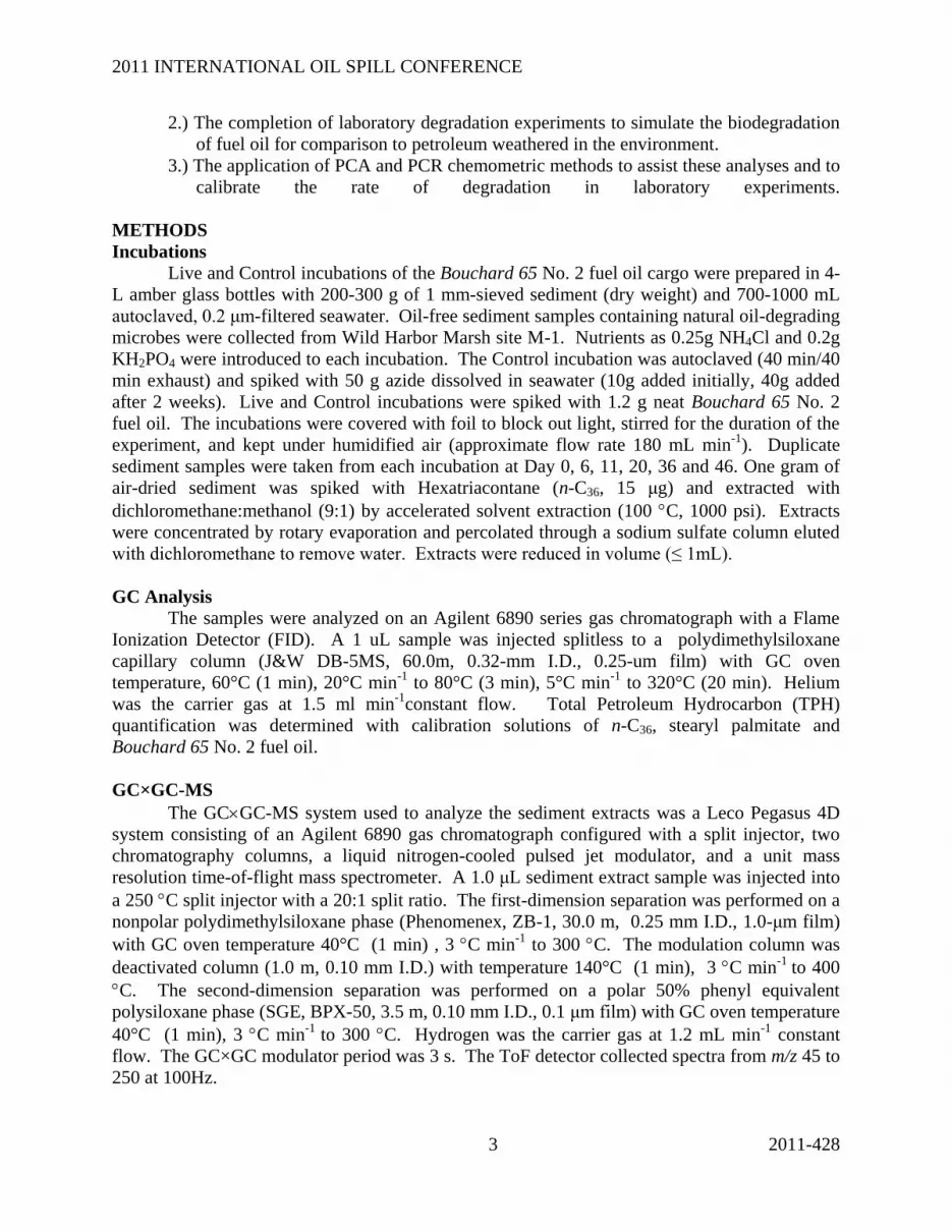
Figure 7. PCA Scores plot for biodegradation time series model. Winsor Cove sample has been

projected onto the model and not used for initial fit.

2011 INTERNATIONAL OIL SPILL CONFERENCE

14 2011-428

Figure 8. PCR for biodegradation time series model. The x-axis is the measured weathering

duration for Live Bouchard 65 oil incubation. The y-axis is predicted weathering from the PCR

model. Regression captured 99.71 percent of the “Y block” variance. Open squares show the

cross-validated fit of each data point to the PCR model with error bars. Winsor Cove sample has

only been predicted, and has been moved to the regression line (approx. 13 days) for

visualization.

2011 INTERNATIONAL OIL SPILL CONFERENCE

15 2011-428

Figure 9. PCR Loadings for biodegradation time series model. Blue peaks in TIC loading (a)

indicate peaks lost during laboratory weathering; red peaks (circled) mark compounds retained

after weathering. Extracted ion m/z 123 loading (b) shows that retained peaks have 123 ion and

belong to sesquiterpane class. GC×GC-MS . Extracted ion m/z 123 data provided for

comparison.

2011 INTERNATIONAL OIL SPILL CONFERENCE

16 2011-428

Table 1 – Mass Spectrum Ions Included in Chemometric Analysis

Chemical Class m/z

Alkanes 57, 71, 85

Acyclic Isoprenoids 113

Alkylcyclohexanes 55, 67, 81, 83, 97

Sesquiterpanes 123, 179, 193, 207

Alkylbenzenes 91, 92, 105, 162, 148, 134, 120

Alkylnaphthalenes 128, 142, 156, 170

Alkylfluoranthenes 166, 180, 194