Page 1
Actuators 2015, 4, 39-59; doi:10.3390/act4010039
actuators ISSN 2076-0825
www.mdpi.com/journal/actuators
Article
Parameters Identification for a Composite Piezoelectric
Actuator Dynamics
Mohammad Saadeh 1,* and Mohamed Trabia 2
1 Department of Computer Science & Industrial Technology, Southeastern Louisiana University,
Hammond, LA 70402-10847, USA 2 Department of Mechanical Engineering, University of Nevada, Las Vegas, NV 89154-4027, USA;
E-Mail: [email protected]
* Author to whom correspondence should be addressed; E-Mail: [email protected] ;
Tel.: +1-985-549-5313; Fax: +1-985-549-5532.
Academic Editors: Mathieu Grossard and Micky Rakotondrabe
Received: 9 January 2015 / Accepted: 11 March 2015 / Published: 17 March 2015
Abstract: This work presents an approach for identifying the model of a composite
piezoelectric (PZT) bimorph actuator dynamics, with the objective of creating a robust
model that can be used under various operating conditions. This actuator exhibits nonlinear
behavior that can be described using backlash and hysteresis. A linear dynamic model with
a damping matrix that incorporates the Bouc–Wen hysteresis model and the backlash
operators is developed. This work proposes identifying the actuator’s model parameters
using the hybrid master-slave genetic algorithm neural network (HGANN). In this algorithm,
the neural network exploits the ability of the genetic algorithm to search globally to optimize
its structure, weights, biases and transfer functions to perform time series analysis efficiently.
A total of nine datasets (cases) representing three different voltage amplitudes excited at
three different frequencies are used to train and validate the model. Four cases are considered
for training the NN architecture, connection weights, bias weights and learning rules. The
remaining five cases are used to validate the model, which produced results that closely
match the experimental ones. The analysis shows that damping parameters are inversely
proportional to the excitation frequency. This indicates that the suggested hysteresis model
is too general for the PZT model in this work. It also suggests that backlash appears only
when dynamic forces become dominant.
OPEN ACCESS
Page 2
Actuators 2015, 4 40
Keywords: piezoelectric bimorph actuator; hybrid genetic algorithms-neural network;
damping; Bouc–Wen hysteresis; backlash
1. Introduction
Recent advances in the area of piezoelectric (PZT) actuators have resulted in their use in many
applications. These actuators are relatively low cost, noninvasive in nature and simple to install. A recent
development is the composite PZT actuators, which use interdigitated electrodes for poling and
subsequent actuation of an internal layer of machined piezoceramic fibers. A thorough discussion of
their characteristics can be found in [1]. Composite PZT actuators have been used in the aviation industry
for controlling various types of aircraft structural members, such as wings [2,3] and fins [4–6].
In [7], they showed that the maximum deflection and axial stresses in the bimorph actuators were
highly dependent on the linearity of the models involved. Some researchers developed control algorithms
based on linear models [8,9]. Their experimental results indicated that the response of the actuator
experienced saturation and asymmetry, which were the results of hysteresis and backlash. Due to the
added complexity associated with modeling hysteresis and backlash in PZT actuators, several
researchers [8–10] used different optimization techniques to model these nonlinear effects. Recently, a
compensation strategy for the asymmetric hysteresis that used two models, connected in series, for
symmetric and asymmetric hysteresis, was proposed [11]. The work in [12] introduced a simple fuzzy
system to model hysteresis in PZT actuators using the inverse of the model, which can be analytically
computed. Another work [13] proposed numerical simulations of the mechanical behavior of a
macro-fiber composite (MFC) actuator shunted by a negative capacitance electronic circuit. They
showed that the elastic parameters of the piezoelectric material can be influenced if a negative
capacitance circuit is connected in parallel to the piezoelectric plate. The authors of [14] introduced a
model to characterize an MFC piezoelectric bimorph actuator that included a generalized Maxwell slip
operator and a creep operator. A finite element model to describe unimorph MFC actuators used in micro
wing models was proposed [3]. In [15], an approximate Galerkin method was used to describe the
relation between the displacement of the MFC actuator’s free end and the amplitude and frequency of
the applied voltage. A finite element method to model an MFC actuator for applications that involve flat
or curved attachments was proposed [16]. Recently, an optimization criteria that can be used for optimal
placement of piezoelectric actuators on laminated structures was introduced [17].
A typical neural network has a fixed architecture and rigid search algorithms that depend on the
number of hidden layers. These issues render typical neural networks computationally intensive; the
search may also be trapped in local minima, which prevents it from performing a generalized search in
a very large space. Several researchers recommended combining genetic algorithms (GA) with neural
networks (NN) to create evolutionary artificial neural networks, which can overcome the typical
limitations of using one of the two methods alone. The suggested synergy between the two approaches
does not only allow the GA to optimize the NN’s weights and biases; it can optimize the architecture of
the NN, as well. In this context, the GA dedicates part of each individual to code the architecture of the
NN (e.g., the number of hidden layers) and iteratively optimizes it.
Page 3
Actuators 2015, 4 41
For example, the work in [18] classified the combination of GA and NN into supportive and
collaborative. In supportive combinations, one of these two algorithms was used first to pre-process data
and to select a few features to be used in the other one. However, the two algorithms were used
simultaneously in the collaborative combinations. Some researchers combined NN learning with GA
paradigms to study how learning can improve genetic search [19,20]. Other researchers [21–24] used
GA to train feed-forward NNs. The work in [25] considered combining neural networks with two genetic
algorithms, the Baldwin effect and the Lamarckian strategy, to study how learning improved the genetic
backpropagation search. Another work [26] addressed the ability of GA in minimizing the resources
used for NN coding. They compared two different genotype encodings that emphasized the compromise
between search space size with fitness landscape and the identification of the associated genetic operators.
A control procedure that used Bayesian NN and GA to solve complex problems while using a hybrid
Monte Carlo method to train the Bayesian networks was proposed [27]. Another work presented a
two-stage approach to improve the performance of the feed-forward neural network [28]. The first stage
of this algorithm deployed a GA search for the best initial weights and biases, while the second stage
included a Newton method to train the network.
The objective of this work is to identify the parameters for the composite piezoelectric bimorph
actuator dynamics that is used in a smart fin design. Similar to earlier researchers, initial observations
show that the behavior of this actuator is nonlinear; it was decided to add backlash and hysteresis
operators to a linear model to describe its behavior accurately. Finding an optimal set of these parameters
of such a model is computationally expensive. In addition, some parameters have extended influence
(i.e., backlash operators also influence the shape of the hysteresis curve). This work uses a hybrid
master-slave genetic algorithm neural network (HGANN) approach [29] to construct a network that can
predict these parameters. A classical back-propagation (BP) network suffers from some inherited
deficiencies. For instance, it takes a longer time to converge [30], and it may converge to local minima,
especially in complex systems [31]. The convergence results are not always guaranteed due to the
monotonic nature of the process [32]. The final results may be biased towards smaller weights [33]. The
BP algorithm is sensitive to the initial parameter’s values [34]. The literature suggested that using GA
for neural network training can overcome most, if not all, problems associated with BP [35,36]. Thus,
this work trains the network using GA that is integrated within a feed-forward NN. The proposed
HGANN algorithm allows the GA to simultaneously train and optimize the network’s topology, transfer
functions, weights and biases. The global nature of the GA search provides the network with better
convergence rates and robust results than the traditional BP, as it searches the entire space domain for
optimal solutions. In addition, mutation improves the GA’s ability to make significant progression
towards an optimal solution, thus saving time and effort without degenerating its converging confidence.
The organization of this work is as follows. The following section describes the prototype of the
actuator and its application in a PZT-actuated smart fin. Then, the dynamic model that incorporates
hysteresis and asymmetrical backlash is presented. The next section presents the use of a HGANN to
identify the parameters for the model. Then, a comparison between the proposed model and experimental
data is included to assess the efficiency of the proposed model. The final section presents the conclusions
of this work.
Page 4
Actuators 2015, 4 42
2. Prototype of the PZT Bimorph Actuator
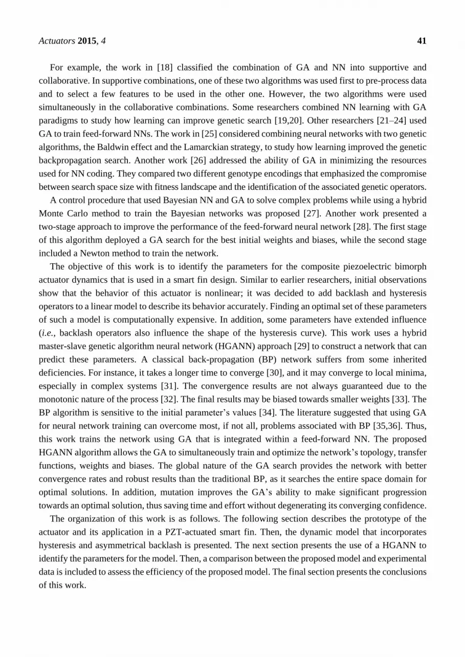
A piezoelectric macro-fiber composite (MFC) actuator is considered in this work. The PZT bimorph
actuator is fabricated by bonding two MFCs [37], as shown in Figure 1. Table 1 summarizes the
properties of the actuator. One MFC is activated in tension by applying positive voltage (along the fiber
axis); while the other MFC is activated in compression by applying negative voltage (against the fiber
axis). The tensile and compressive strains induce a distributed couple that causes the actuator to bend.
The actuator can bend in the reverse direction by changing the polarity of the input voltages.
Figure 1. Geometry of a piezoelectric (PZT) bimorph actuator.
Table 1. Characteristics of the PZT bimorph actuator. MFC, macro-fiber composite.
Variable Fiberglass MFC
Length (mm) Lf = 17 Lp = 85 (active length)
Width (mm) bf = 75 bp = 56
Height (mm) hf = 0.5 hp = 0.3
PZT strain constant d33 (m/V) N/A d33 = 4.275 × 10⁻¹⁰
Electrode spacing es (mm) N/A es = 0.5
3. PZT Bimorph-Actuated Smart Fin
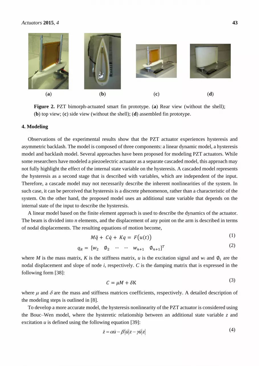
To assess the effectiveness of the PZT bimorph actuator, it is incorporated into a smart fin design,
which can be used to either steer or stabilize an aerial vehicle. The fin has a rigid hollow shell that rotates
around an axle, which is fixed to the body of the vehicle. The actuator is completely enclosed within the
fin, as shown in Figure 2. The bending of the PZT actuator is used to control the orientation of the fin.
One end of the actuator is rigidly connected to the axle of the fin. The other end passes through a slot in
a hinge that is placed at the tip of the fin. This arrangement allows the actuator to slide freely within the
slot without binding when activated. A through-shaft incremental encoder is used to measure the rotation
angle of the smart fin.
Lp
Lf
2hp
bp
bf Lf
Page 5
Actuators 2015, 4 43
(a) (b) (c) (d)
Figure 2. PZT bimorph-actuated smart fin prototype. (a) Rear view (without the shell);
(b) top view; (c) side view (without the shell); (d) assembled fin prototype.
4. Modeling
Observations of the experimental results show that the PZT actuator experiences hysteresis and
asymmetric backlash. The model is composed of three components: a linear dynamic model, a hysteresis
model and backlash model. Several approaches have been proposed for modeling PZT actuators. While
some researchers have modeled a piezoelectric actuator as a separate cascaded model, this approach may
not fully highlight the effect of the internal state variable on the hysteresis. A cascaded model represents
the hysteresis as a second stage that is described with variables, which are independent of the input.
Therefore, a cascade model may not necessarily describe the inherent nonlinearities of the system. In
such case, it can be perceived that hysteresis is a discrete phenomenon, rather than a characteristic of the
system. On the other hand, the proposed model uses an additional state variable that depends on the
internal state of the input to describe the hysteresis.
A linear model based on the finite element approach is used to describe the dynamics of the actuator.
The beam is divided into n elements, and the displacement of any point on the arm is described in terms
of nodal displacements. The resulting equations of motion become,
𝑀�̈� + 𝐶�̇� + 𝐾𝑞 = 𝐹(𝑢(𝑡)) (1)
𝑞𝑅 = [𝑤2 ∅2… … 𝑤𝑛+1 ∅𝑛+1]
𝑇 (2)
where M is the mass matrix, K is the stiffness matrix, u is the excitation signal and wi and ∅i are the
nodal displacement and slope of node i, respectively. C is the damping matrix that is expressed in the
following form [38]:
𝐶 = 𝜇𝑀 + 𝛿K (3)
where and are the mass and stiffness matrices coefficients, respectively. A detailed description of
the modeling steps is outlined in [8].
To develop a more accurate model, the hysteresis nonlinearity of the PZT actuator is considered using
the Bouc–Wen model, where the hysteretic relationship between an additional state variable z and
excitation u is defined using the following equation [39]:
zuzuuz (4)
Page 6
Actuators 2015, 4 44
where , and are the parameters that determine the magnitude and shape of the hysteresis loop. The
state variable z is incorporated into Equation (1) as follows,
𝑀�̈� + 𝐶�̇� + 𝐾𝑞 = 𝐹(𝑢(𝑡)) − 𝑒∗𝑇𝑧 (5)
where e*T is a unit vector whose (2n−1)-th element is one and the remaining elements are zeros (where
n is the number of elements).
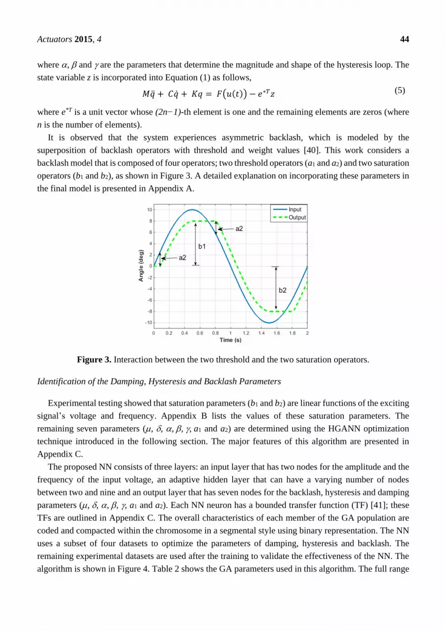
It is observed that the system experiences asymmetric backlash, which is modeled by the
superposition of backlash operators with threshold and weight values [40]. This work considers a
backlash model that is composed of four operators; two threshold operators (a1 and a2) and two saturation
operators (b1 and b2), as shown in Figure 3. A detailed explanation on incorporating these parameters in
the final model is presented in Appendix A.
Figure 3. Interaction between the two threshold and the two saturation operators.
Identification of the Damping, Hysteresis and Backlash Parameters
Experimental testing showed that saturation parameters (b1 and b2) are linear functions of the exciting
signal’s voltage and frequency. Appendix B lists the values of these saturation parameters. The
remaining seven parameters (, , ,,,a1 and a2) are determined using the HGANN optimization
technique introduced in the following section. The major features of this algorithm are presented in
Appendix C.
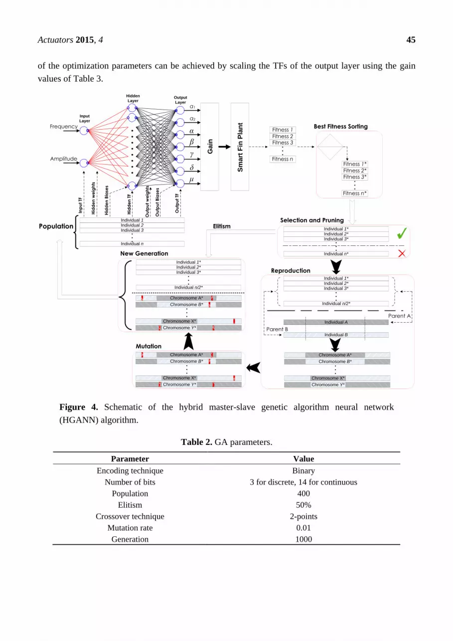
The proposed NN consists of three layers: an input layer that has two nodes for the amplitude and the
frequency of the input voltage, an adaptive hidden layer that can have a varying number of nodes
between two and nine and an output layer that has seven nodes for the backlash, hysteresis and damping
parameters (,, ,, , a1 and a2). Each NN neuron has a bounded transfer function (TF) [41]; these
TFs are outlined in Appendix C. The overall characteristics of each member of the GA population are
coded and compacted within the chromosome in a segmental style using binary representation. The NN
uses a subset of four datasets to optimize the parameters of damping, hysteresis and backlash. The
remaining experimental datasets are used after the training to validate the effectiveness of the NN. The
algorithm is shown in Figure 4. Table 2 shows the GA parameters used in this algorithm. The full range
Page 7
Actuators 2015, 4 45
of the optimization parameters can be achieved by scaling the TFs of the output layer using the gain
values of Table 3.
Figure 4. Schematic of the hybrid master-slave genetic algorithm neural network
(HGANN) algorithm.
Table 2. GA parameters.
Parameter Value
Encoding technique Binary
Number of bits 3 for discrete, 14 for continuous
Population 400
Elitism 50%
Crossover technique 2-points
Mutation rate 0.01
Generation 1000
Input
Layer
Hidden
LayerOutput
Layer
α
β
γ
δ
μ
a1
a2
Ga
in
Sm
art
Fin
Pla
nt
. . . . . . . .Frequency
Amplitude
PopulationIndividual 1Individual 2Individual 3
Individual n
. . .
Fitness 1
Fitness 2Fitness 3
. . .
Individual 1*Individual 2*Individual 3*
Individual n*
. . .
Individual 1*Individual 2*Individual 3*
. . .
Individual n/2*
Individual A
Individual B
Parent A
Parent B
Chromosome A*
Chromosome B*
Individual 1*Individual 2*Individual 3*
. . .
Individual n/2*
. . .
Chromosome X*
Chromosome Y*
Fitness nFitness 1*
Fitness 2*Fitness 3*
. . .
Fitness n*
Chromosome A*
Chromosome B*
. . .
Chromosome X*
Chromosome Y*
Chromosome A*
Chromosome B*
. . .
Chromosome X*
Chromosome Y*
Best Fitness Sorting
Selection and Pruning
Reproduction
Mutation
New Generation
Elitism
Inp
ut
TF
Hid
de
n w
eig
hts
Hid
de
n B
iase
s
Ou
tpu
t B
iase
s
Hid
de
n T
F
Ou
tpu
t w
eig
hts
Ou
tpu
t TF
Page 8
Actuators 2015, 4 46
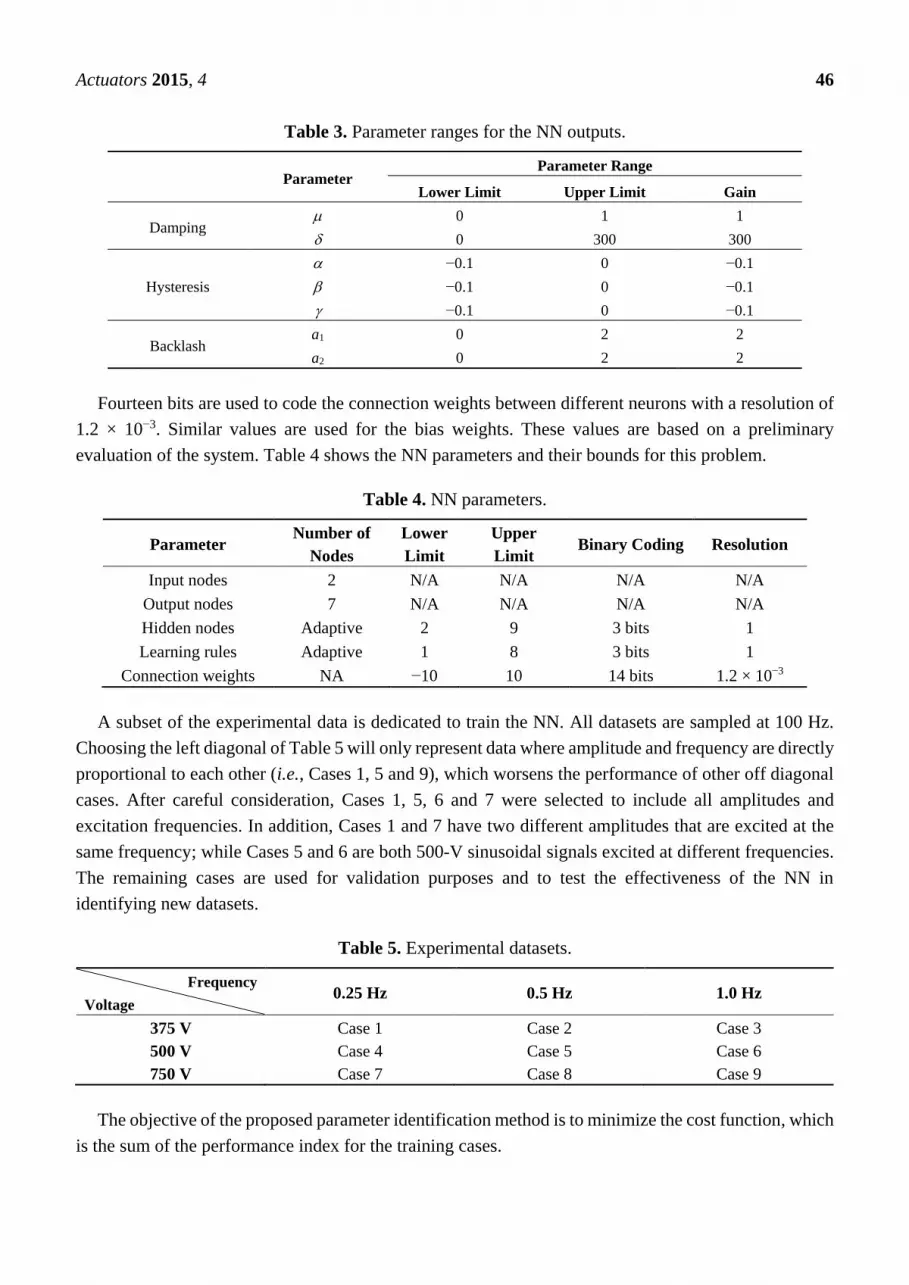
Table 3. Parameter ranges for the NN outputs.
Parameter Parameter Range
Lower Limit Upper Limit Gain
Damping 0 1 1
0 300 300
Hysteresis
−0.1 0 −0.1
−0.1 0 −0.1
−0.1 0 −0.1
Backlash a1 0 2 2
a2 0 2 2
Fourteen bits are used to code the connection weights between different neurons with a resolution of
1.2 × 10⁻³. Similar values are used for the bias weights. These values are based on a preliminary
evaluation of the system. Table 4 shows the NN parameters and their bounds for this problem.
Table 4. NN parameters.
Parameter Number of
Nodes
Lower
Limit
Upper
Limit Binary Coding Resolution
Input nodes 2 N/A N/A N/A N/A
Output nodes 7 N/A N/A N/A N/A
Hidden nodes Adaptive 2 9 3 bits 1
Learning rules Adaptive 1 8 3 bits 1
Connection weights NA −10 10 14 bits 1.2 × 10⁻³
A subset of the experimental data is dedicated to train the NN. All datasets are sampled at 100 Hz.
Choosing the left diagonal of Table 5 will only represent data where amplitude and frequency are directly
proportional to each other (i.e., Cases 1, 5 and 9), which worsens the performance of other off diagonal
cases. After careful consideration, Cases 1, 5, 6 and 7 were selected to include all amplitudes and
excitation frequencies. In addition, Cases 1 and 7 have two different amplitudes that are excited at the
same frequency; while Cases 5 and 6 are both 500-V sinusoidal signals excited at different frequencies.
The remaining cases are used for validation purposes and to test the effectiveness of the NN in
identifying new datasets.
Table 5. Experimental datasets.
Frequency
Voltage 0.25 Hz 0.5 Hz 1.0 Hz
375 V Case 1 Case 2 Case 3
500 V Case 4 Case 5 Case 6
750 V Case 7 Case 8 Case 9
The objective of the proposed parameter identification method is to minimize the cost function, which
is the sum of the performance index for the training cases.
Page 9
Actuators 2015, 4 47
𝐶𝐹 = ∑𝑃𝐼𝐶 = ∑(∑(𝛽exp(𝑖) − 𝛽𝑚𝑜𝑑(𝑖))2
𝑛
𝑖=1
)
𝐶
𝐶 = 1,5,6,7 (6)
where CF is the sum of squared errors, PI is the performance index for each case, n is the total number
of data samples, βexp(i) is the measured fin angle at the i-th sample and βmod(i) is the fin angle produced
by the dynamic model at the same i-th sample.
5. Results
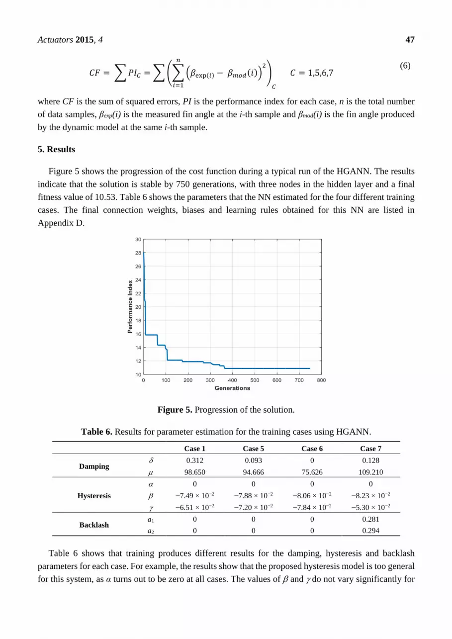
Figure 5 shows the progression of the cost function during a typical run of the HGANN. The results
indicate that the solution is stable by 750 generations, with three nodes in the hidden layer and a final
fitness value of 10.53. Table 6 shows the parameters that the NN estimated for the four different training
cases. The final connection weights, biases and learning rules obtained for this NN are listed in
Appendix D.
Figure 5. Progression of the solution.
Table 6. Results for parameter estimation for the training cases using HGANN.
Case 1 Case 5 Case 6 Case 7
Damping 0.312 0.093 0 0.128
98.650 94.666 75.626 109.210
Hysteresis
0 0 0 0
−7.49 × 10⁻² −7.88 × 10⁻² −8.06 × 10⁻² −8.23 × 10⁻²
−6.51 × 10⁻² −7.20 × 10⁻² −7.84 × 10⁻² −5.30 × 10⁻²
Backlash a1 0 0 0 0.281
a2 0 0 0 0.294
Table 6 shows that training produces different results for the damping, hysteresis and backlash
parameters for each case. For example, the results show that the proposed hysteresis model is too general
for this system, as α turns out to be zero at all cases. The values of and do not vary significantly for
Page 10
Actuators 2015, 4 48
the four training cases. On the other side, the values of the damping coefficients, and , differ for each
case. The results also show that the backlash operators are only active in Case 7.
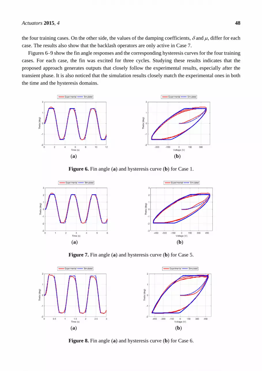
Figures 6–9 show the fin angle responses and the corresponding hysteresis curves for the four training
cases. For each case, the fin was excited for three cycles. Studying these results indicates that the
proposed approach generates outputs that closely follow the experimental results, especially after the
transient phase. It is also noticed that the simulation results closely match the experimental ones in both
the time and the hysteresis domains.
(a)
(b)
Figure 6. Fin angle (a) and hysteresis curve (b) for Case 1.
(a)
(b)
Figure 7. Fin angle (a) and hysteresis curve (b) for Case 5.
(a)
(b)
Figure 8. Fin angle (a) and hysteresis curve (b) for Case 6.
Page 11
Actuators 2015, 4 49
(a)
(b)
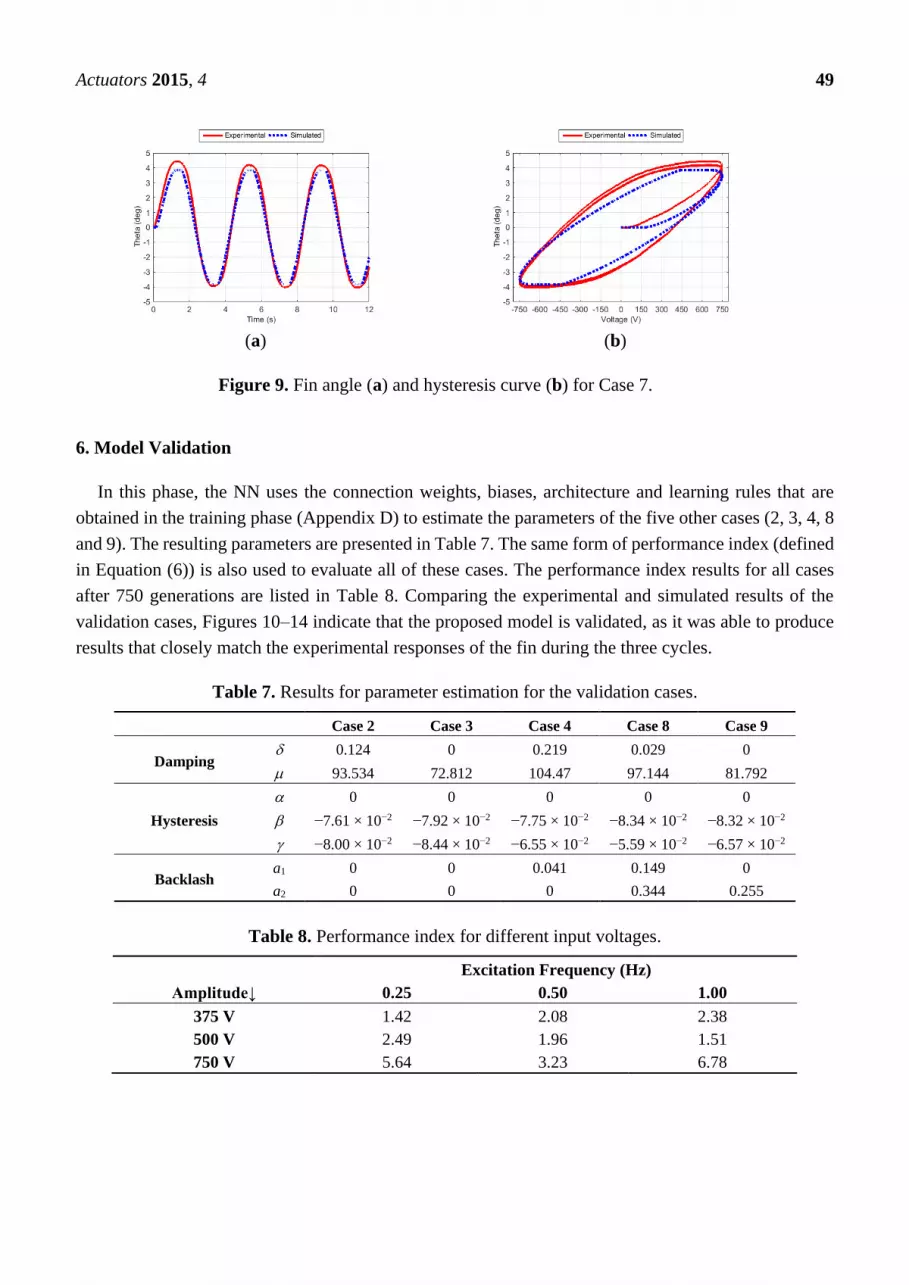
Figure 9. Fin angle (a) and hysteresis curve (b) for Case 7.
6. Model Validation
In this phase, the NN uses the connection weights, biases, architecture and learning rules that are
obtained in the training phase (Appendix D) to estimate the parameters of the five other cases (2, 3, 4, 8
and 9). The resulting parameters are presented in Table 7. The same form of performance index (defined
in Equation (6)) is also used to evaluate all of these cases. The performance index results for all cases
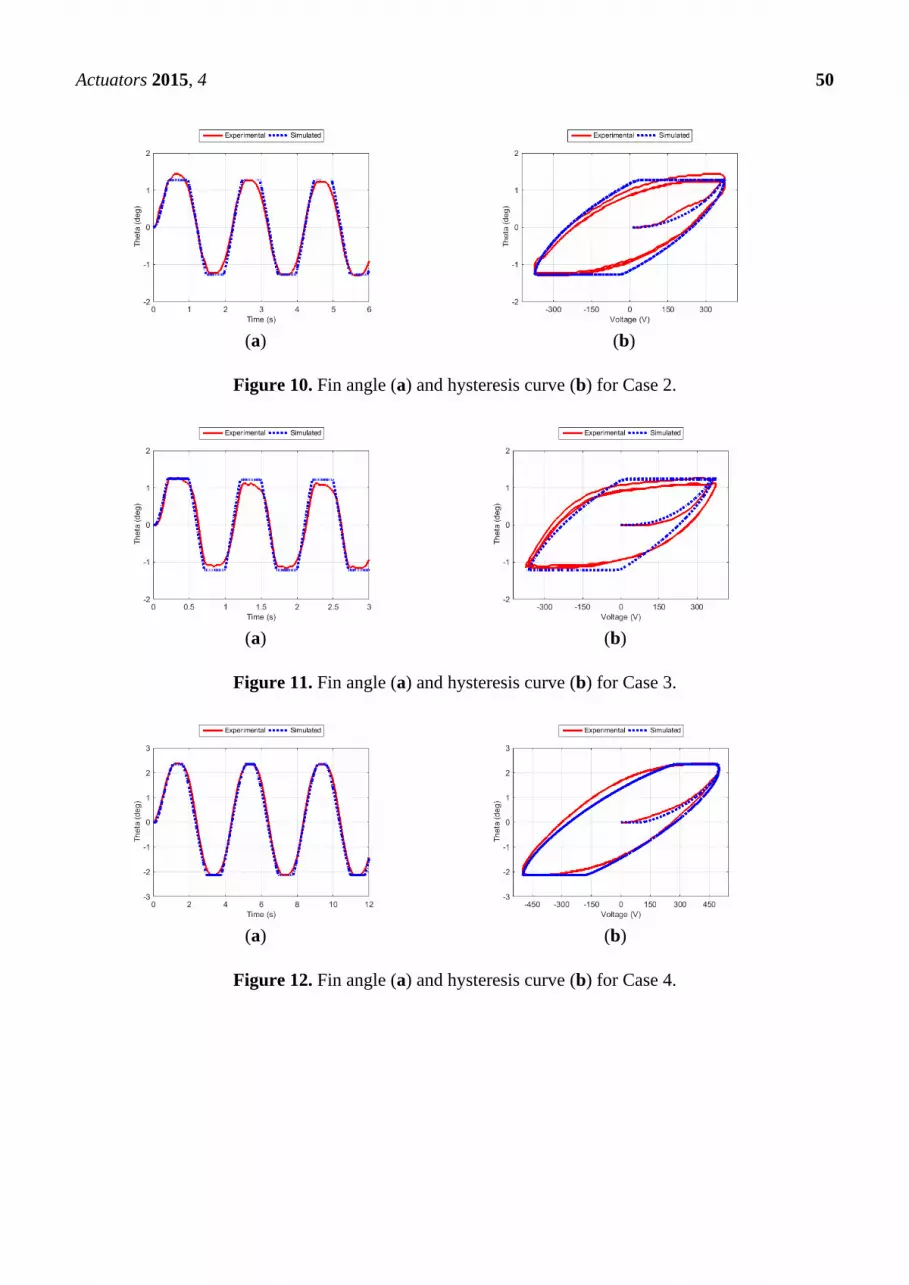
after 750 generations are listed in Table 8. Comparing the experimental and simulated results of the
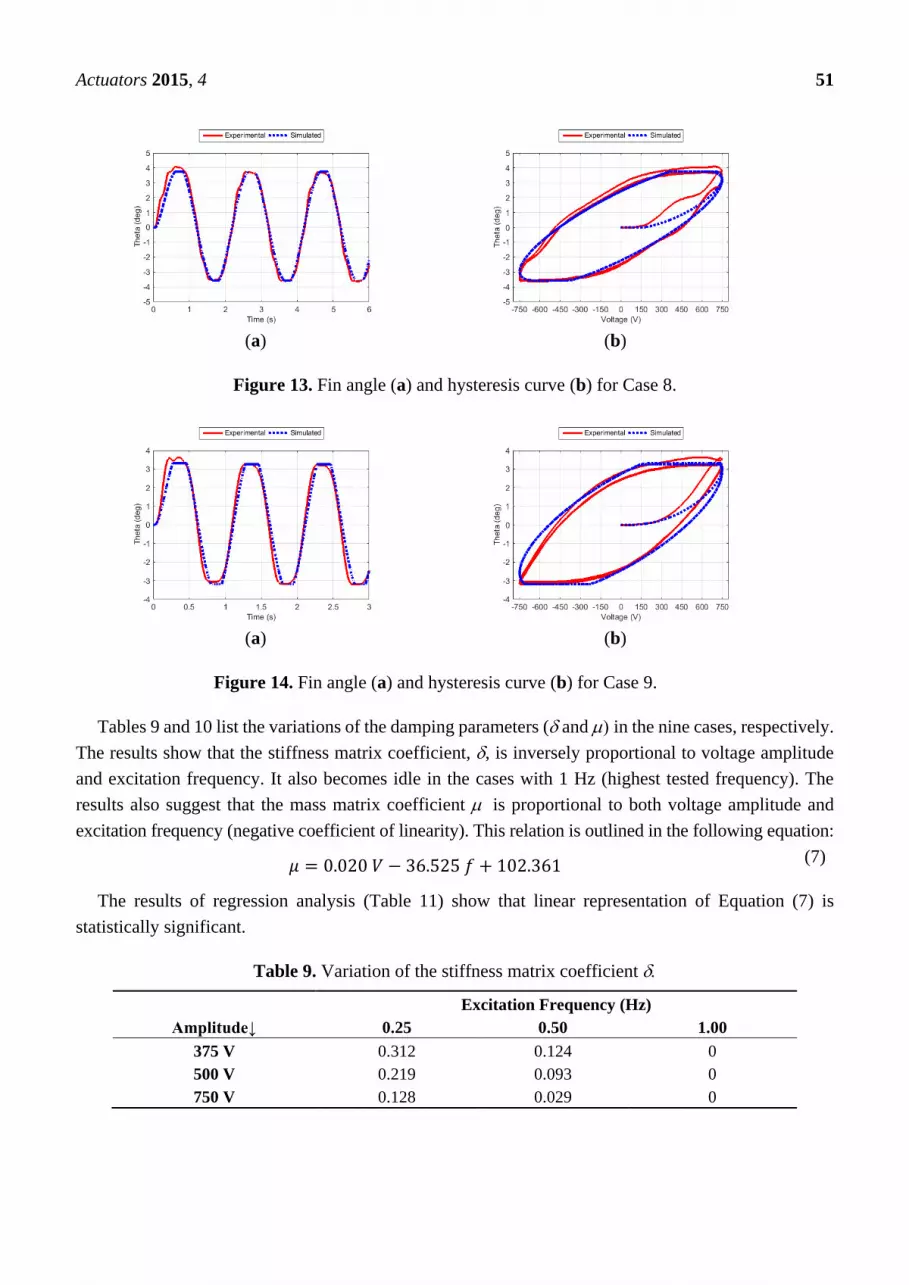
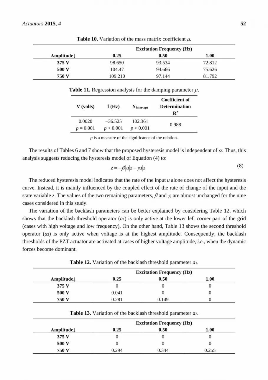
validation cases, Figures 10–14 indicate that the proposed model is validated, as it was able to produce
results that closely match the experimental responses of the fin during the three cycles.
Table 7. Results for parameter estimation for the validation cases.
Case 2 Case 3 Case 4 Case 8 Case 9
Damping 0.124 0 0.219 0.029 0
93.534 72.812 104.47 97.144 81.792
Hysteresis
0 0 0 0 0
−7.61 × 10⁻² −7.92 × 10⁻² −7.75 × 10⁻² −8.34 × 10⁻² −8.32 × 10⁻²
−8.00 × 10⁻² −8.44 × 10⁻² −6.55 × 10⁻² −5.59 × 10⁻² −6.57 × 10⁻²
Backlash a1 0 0 0.041 0.149 0
a2 0 0 0 0.344 0.255
Table 8. Performance index for different input voltages.
Excitation Frequency (Hz)
Amplitude↓ 0.25 0.50 1.00
375 V 1.42 2.08 2.38
500 V 2.49 1.96 1.51
750 V 5.64 3.23 6.78
Page 12
Actuators 2015, 4 50
(a)
(b)
Figure 10. Fin angle (a) and hysteresis curve (b) for Case 2.
(a)
(b)
Figure 11. Fin angle (a) and hysteresis curve (b) for Case 3.
(a)
(b)
Figure 12. Fin angle (a) and hysteresis curve (b) for Case 4.
Page 13
Actuators 2015, 4 51
(a)
(b)
Figure 13. Fin angle (a) and hysteresis curve (b) for Case 8.
(a)
(b)
Figure 14. Fin angle (a) and hysteresis curve (b) for Case 9.
Tables 9 and 10 list the variations of the damping parameters ( and in the nine cases, respectively.
The results show that the stiffness matrix coefficient, , is inversely proportional to voltage amplitude
and excitation frequency. It also becomes idle in the cases with 1 Hz (highest tested frequency). The
results also suggest that the mass matrix coefficient is proportional to both voltage amplitude and
excitation frequency (negative coefficient of linearity). This relation is outlined in the following equation:
𝜇 = 0.020 𝑉 − 36.525 𝑓 + 102.361 (7)
The results of regression analysis (Table 11) show that linear representation of Equation (7) is
statistically significant.
Table 9. Variation of the stiffness matrix coefficient
Excitation Frequency (Hz)
Amplitude↓ 0.25 0.50 1.00
375 V 0.312 0.124 0
500 V 0.219 0.093 0
750 V 0.128 0.029 0
Page 14
Actuators 2015, 4 52
Table 10. Variation of the mass matrix coefficient
Excitation Frequency (Hz)
Amplitude↓ 0.25 0.50 1.00
375 V 98.650 93.534 72.812
500 V 104.47 94.666 75.626
750 V 109.210 97.144 81.792
Table 11. Regression analysis for the damping parameter .
V (volts) f (Hz) Yintercept
Coefficient of
Determination
R2
0.0020
p = 0.001
−36.525
p < 0.001
102.361
p < 0.001 0.988
p is a measure of the significance of the relation.
The results of Tables 6 and 7 show that the proposed hysteresis model is independent of . Thus, this
analysis suggests reducing the hysteresis model of Equation (4) to:
zuzuz (8)
The reduced hysteresis model indicates that the rate of the input u alone does not affect the hysteresis
curve. Instead, it is mainly influenced by the coupled effect of the rate of change of the input and the
state variable z. The values of the two remaining parameters, and , are almost unchanged for the nine
cases considered in this study.
The variation of the backlash parameters can be better explained by considering Table 12, which
shows that the backlash threshold operator (a1) is only active at the lower left corner part of the grid
(cases with high voltage and low frequency). On the other hand, Table 13 shows the second threshold
operator (a2) is only active when voltage is at the highest amplitude. Consequently, the backlash
thresholds of the PZT actuator are activated at cases of higher voltage amplitude, i.e., when the dynamic
forces become dominant.
Table 12. Variation of the backlash threshold parameter a1.
Excitation Frequency (Hz)
Amplitude↓ 0.25 0.50 1.00
375 V 0 0 0
500 V 0.041 0 0
750 V 0.281 0.149 0
Table 13. Variation of the backlash threshold parameter a2.
Excitation Frequency (Hz)
Amplitude↓ 0.25 0.50 1.00
375 V 0 0 0
500 V 0 0 0
750 V 0.294 0.344 0.255
Page 15
Actuators 2015, 4 53
7. Conclusions
This work presents an approach for the identification of a composite piezoelectric (PZT) bimorph
actuator. As an example for application, the actuator is incorporated within a smart fin prototype. The
novelty of the work lies in proposing an approach to use a hybrid neural network to model the behavior
of a PZT actuator that does not only mimic a specific behavior, but is also able to predict the behavior
under different voltage and excitation frequency. The performance of the actuator is considered for nine
test cases that represent three voltage amplitudes (375, 500 and 750 V) excited at three different
frequencies (0.25, 0.50 and 1.0 Hz).
Similar to earlier research in this area, it is observed that the actuator experiences hysteresis and
backlash. The system is modeled using a linear dynamic model. A damping matrix, the Bouc–Wen
hysteresis model and backlash operators are also included in the model. Full identification of the actuator
model is needed to predict the performance of the actuator and to utilize it in control schemes.
While it is easy to estimate the values of the saturation operators of the backlash model based on
experimental results, it may not be intuitive to determine the correct values of the threshold parameters
of the model. A hybrid neural network genetic algorithm (HGANN) is used for identification of the
remaining parameters of the model. HGANN allows genetic algorithm to simultaneously tune the
weights and learning rules of the neural network representing the model and to adjust the structure of its
hidden layer, such that the cost function can be minimized. In this work, four sinusoidal inputs of mixed
amplitudes and frequencies are used to train the NN’s biases, weights and learning rules. The other five
cases are left for validating the performance of the NN and its robustness to input variations. Comparing
the experimental and simulation results of the training cases indicates that the neural network obtained
from the training is robust enough to handle multiple operating conditions. Additionally, the robustness
of the resulting neural network is verified by its satisfactory performance when applied to each of the
remaining five cases.
It may be insightful to study the values of the model parameters in the nine cases to understand the
nature of the proposed model. For example, the two damping parameters show that the coefficient of the
stiffness matrix, , is inversely proportional to the voltage amplitude and excitation frequency. The effect
of the stiffness matrix disappears completely in the highest frequency cases (1-Hz cases). On the other
hand, the results show that the coefficient of the mass matrix, , is proportional to the voltage amplitude
and inversely proportional to the excitation frequency. The results also indicate that the hysteresis model
is too general for the composite piezoelectric bimorph actuator model, since the rate of change of the
input signal (�̇�) does not influence the hysteresis curve. The remaining two parameters ( and ) are
reasonably consistent for all nine cases, which show the limited sensitivity of the proposed hysteresis
model to changes in exciting voltage and frequency. It is observed that the two backlash threshold
operators are only active in the cases of high voltage amplitude. The results suggest that backlash appears
only when dynamic forces become dominant.
Acknowledgments
This work was partially supported by the U.S. Army Research Laboratory (DAAD19-03-2-0007).
Page 16
Actuators 2015, 4 54
Author Contributions
Mohamed Trabia designed the experiments. Mohammad Saadeh performed the experiments and
developed the HGANN. Mohammad Saadeh and Mohamed Trabia analyzed the data and wrote
the paper.
Conflicts of Interest
The authors declare no conflict of interest.
Appendix
Appendix A: Backlash Operators
It is known that complex hysteretic nonlinearity is better modeled by the superposition of many
backlash operators with different threshold and weight values [40]. To accurately represent the backlash
of the fin prototype, it was decided to use four operators; two threshold operators (a1 and a2) and two
saturation operators (b1 and b2). These backlash operators work as follows:
Assuming that the process starts at zero initial condition, the output remains zero until the input
reaches the threshold value of a1, which is the control input’s first threshold value. The hysteresis
operator at this stage is:
)(
,)(min
,)(
max)( 1
1
tty
atx
atx
ty
(A1)
The threshold operator, a1, continues to be active until a saturation operator, b1, is reached. The output
remains equal to this saturation value. The above equation becomes:
)(
,)(min
,)(
max
,
min)(1
1
1
tty
atx
atx
b
ty
(A2)
The output remains equal to b1 until the second backlash operator, a2, is activated as follows:
)(
,)(min
,)(
max)(
,
)(
,)(min
,)(
max
2
2
12
2
tty
atx
atx
ty
then
b
tty
atx
atx
if
(A3)
The second backlash operator remains in effect until the second saturation value, b2, is reached. At
this stage, the output is equal to,
Page 17
Actuators 2015, 4 55
)(
,)(min
,)(
max
,
min)(2
2
2
tty
atx
atx
b
ty
(A4)
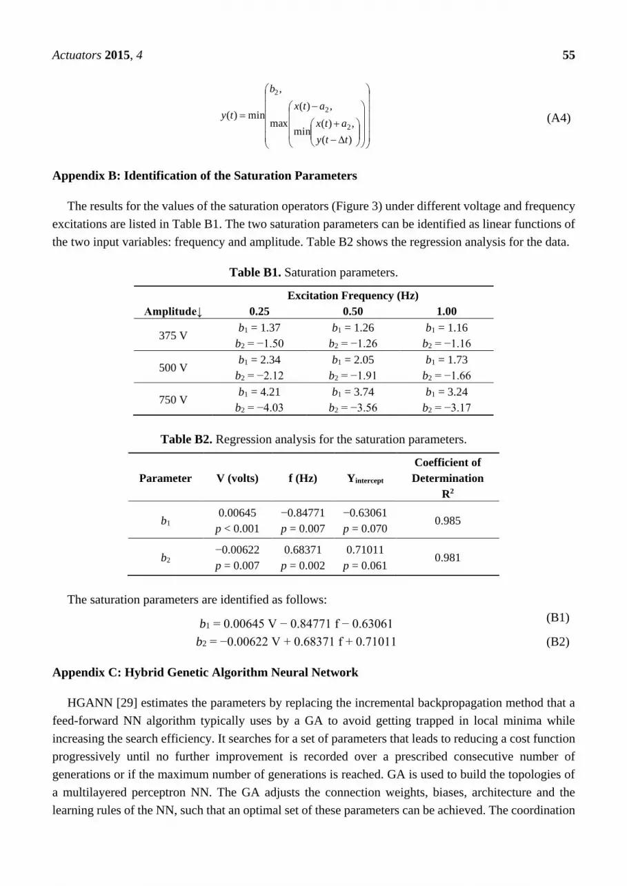
Appendix B: Identification of the Saturation Parameters
The results for the values of the saturation operators (Figure 3) under different voltage and frequency
excitations are listed in Table B1. The two saturation parameters can be identified as linear functions of
the two input variables: frequency and amplitude. Table B2 shows the regression analysis for the data.
Table B1. Saturation parameters.
Excitation Frequency (Hz)
Amplitude↓ 0.25 0.50 1.00
375 V b1 = 1.37
b2 = −1.50
b1 = 1.26
b2 = −1.26
b1 = 1.16
b2 = −1.16
500 V b1 = 2.34
b2 = −2.12
b1 = 2.05
b2 = −1.91
b1 = 1.73
b2 = −1.66
750 V b1 = 4.21
b2 = −4.03
b1 = 3.74
b2 = −3.56
b1 = 3.24
b2 = −3.17
Table B2. Regression analysis for the saturation parameters.
Parameter V (volts) f (Hz) Yintercept
Coefficient of
Determination
R2
b1 0.00645
p < 0.001
−0.84771
p = 0.007
−0.63061
p = 0.070 0.985
b2 −0.00622
p = 0.007
0.68371
p = 0.002
0.71011
p = 0.061 0.981
The saturation parameters are identified as follows:
b1 = 0.00645 V − 0.84771 f − 0.63061 (B1)
b2 = −0.00622 V + 0.68371 f + 0.71011 (B2)
Appendix C: Hybrid Genetic Algorithm Neural Network
HGANN [29] estimates the parameters by replacing the incremental backpropagation method that a
feed-forward NN algorithm typically uses by a GA to avoid getting trapped in local minima while
increasing the search efficiency. It searches for a set of parameters that leads to reducing a cost function
progressively until no further improvement is recorded over a prescribed consecutive number of
generations or if the maximum number of generations is reached. GA is used to build the topologies of
a multilayered perceptron NN. The GA adjusts the connection weights, biases, architecture and the
learning rules of the NN, such that an optimal set of these parameters can be achieved. The coordination
Page 18
Actuators 2015, 4 56
between GA and NN provides the proposed algorithm with flexibility that increases the search efficiency
through the parallel adjustment of many NN features simultaneously. The algorithm can be summarized
as follows:
1. Generate a random initial population where the NN characteristics are coded into the genetic
material of each individual.
2. Expand the compacted information of each individual and decode the genetic material into neural
material, including; connection weights, biases, architecture and learning rules.
3. Feed the four training cases for each individual at the input layer to identify the parameters of
damping, hysteresis and backlash.
4. Feed the parameters obtained at Step (3) into the dynamic model of the actuator to generate the
simulated output angle.
5. Evaluate the fitness of each individual. The individuals are then rearranged according to
their fitness.
6. Prune the least fitted individuals and select the best fitted ones as members of the new generation,
as well as parents who will undergo the reproduction phases of crossover and mutation to produce new
offspring for the next generation.
7. Combine the new offspring with the best fitted individuals of the current generation to establish
the population of the new generation.
8. Repeat Steps 2 through 7 to progressively optimize a cost function until either the maximum
number of generations is reached or there is no significant improvement recorded within the previous
200 successive generations.
Each NN neuron has a transfer function (TF), which maps the overall inputs of the neuron into a
different output space. These TFs are found in all layers; input, hidden and output. This algorithm uses
unitary bounded neural TFs: hardlim, hardlims, satlin, satlins, tribas, tansig, logsig and radbas, as defined
in the MATLAB Neural Networks Toolbox [41]. These TFs are randomly coded in the GA individuals,
which iteratively searches for the optimal selection out of these TFs. Each of the TFs is identified in the
genetic material using a number between one and eight.
The impacts that some neurons have on others depend on the connection weights. Besides connection
weights, a neuron has a bias input that helps the neuron exceed its threshold and fire regardless of the
other inputs values. A bias always fires a unit input that is scaled by a weight, which is determined by
the GA. All weights are continuous and range between (−10 and 10).
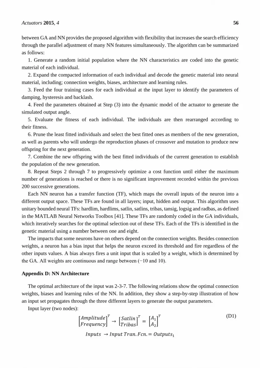
Appendix D: NN Architecture
The optimal architecture of the input was 2-3-7. The following relations show the optimal connection
weights, biases and learning rules of the NN. In addition, they show a step-by-step illustration of how
an input set propagates through the three different layers to generate the output parameters.
Input layer (two nodes):
[𝐴𝑚𝑝𝑙𝑖𝑡𝑢𝑑𝑒𝐹𝑟𝑒𝑞𝑢𝑒𝑛𝑐𝑦
]𝑇
→ [𝑆𝑎𝑡𝑙𝑖𝑛𝑇𝑟𝑖𝑏𝑎𝑠
]𝑇
= [𝐴1
𝐴2]𝑇
(D1)
𝐼𝑛𝑝𝑢𝑡𝑠 → 𝐼𝑛𝑝𝑢𝑡 𝑇𝑟𝑎𝑛. 𝐹𝑐𝑛.= 𝑂𝑢𝑡𝑝𝑢𝑡𝑠1
Page 19
Actuators 2015, 4 57
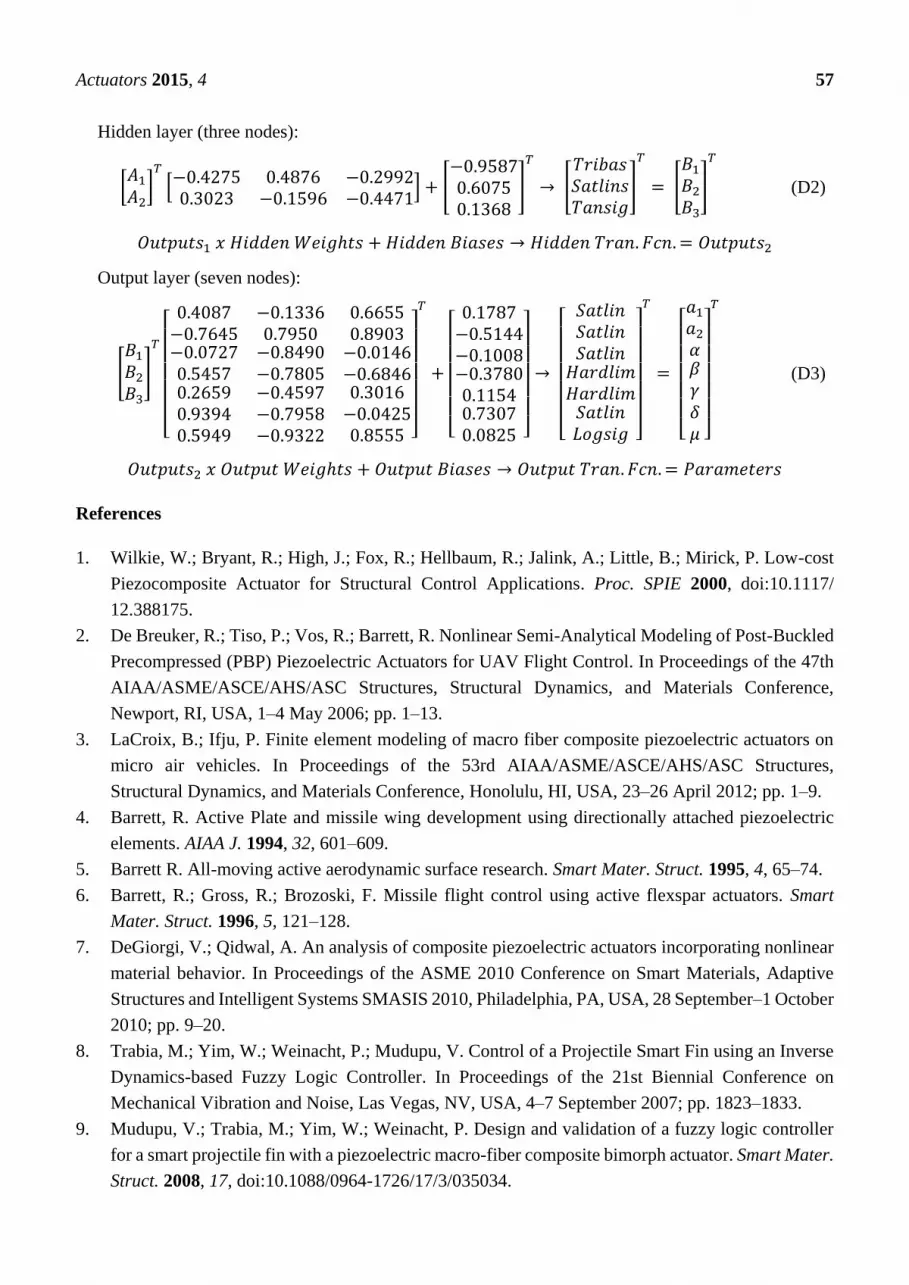
Hidden layer (three nodes):
[𝐴1
𝐴2]𝑇
[−0.4275 0.4876 −0.29920.3023 −0.1596 −0.4471
] + [−0.95870.60750.1368
]
𝑇
→ [𝑇𝑟𝑖𝑏𝑎𝑠𝑆𝑎𝑡𝑙𝑖𝑛𝑠𝑇𝑎𝑛𝑠𝑖𝑔
]
𝑇
= [𝐵1
𝐵2
𝐵3
]
𝑇
(D2)
𝑂𝑢𝑡𝑝𝑢𝑡𝑠1 𝑥 𝐻𝑖𝑑𝑑𝑒𝑛 𝑊𝑒𝑖𝑔ℎ𝑡𝑠 + 𝐻𝑖𝑑𝑑𝑒𝑛 𝐵𝑖𝑎𝑠𝑒𝑠 → 𝐻𝑖𝑑𝑑𝑒𝑛 𝑇𝑟𝑎𝑛. 𝐹𝑐𝑛.= 𝑂𝑢𝑡𝑝𝑢𝑡𝑠2
Output layer (seven nodes):
[𝐵1
𝐵2
𝐵3
]
𝑇
[
0.4087 −0.1336 0.6655−0.7645 0.7950 0.8903−0.07270.54570.26590.93940.5949
−0.8490−0.7805−0.4597−0.7958−0.9322
−0.0146−0.68460.3016
−0.04250.8555 ]
𝑇
+
[
0.1787−0.5144−0.1008−0.37800.11540.73070.0825 ]
→
[
𝑆𝑎𝑡𝑙𝑖𝑛𝑆𝑎𝑡𝑙𝑖𝑛𝑆𝑎𝑡𝑙𝑖𝑛
𝐻𝑎𝑟𝑑𝑙𝑖𝑚𝐻𝑎𝑟𝑑𝑙𝑖𝑚𝑆𝑎𝑡𝑙𝑖𝑛𝐿𝑜𝑔𝑠𝑖𝑔 ]
𝑇
=
[ 𝑎1
𝑎2
𝛼𝛽𝛾𝛿𝜇 ]
𝑇
(D3)
𝑂𝑢𝑡𝑝𝑢𝑡𝑠2 𝑥 𝑂𝑢𝑡𝑝𝑢𝑡 𝑊𝑒𝑖𝑔ℎ𝑡𝑠 + 𝑂𝑢𝑡𝑝𝑢𝑡 𝐵𝑖𝑎𝑠𝑒𝑠 → 𝑂𝑢𝑡𝑝𝑢𝑡 𝑇𝑟𝑎𝑛. 𝐹𝑐𝑛.= 𝑃𝑎𝑟𝑎𝑚𝑒𝑡𝑒𝑟𝑠
References
1. Wilkie, W.; Bryant, R.; High, J.; Fox, R.; Hellbaum, R.; Jalink, A.; Little, B.; Mirick, P. Low-cost
Piezocomposite Actuator for Structural Control Applications. Proc. SPIE 2000, doi:10.1117/
12.388175.
2. De Breuker, R.; Tiso, P.; Vos, R.; Barrett, R. Nonlinear Semi-Analytical Modeling of Post-Buckled
Precompressed (PBP) Piezoelectric Actuators for UAV Flight Control. In Proceedings of the 47th
AIAA/ASME/ASCE/AHS/ASC Structures, Structural Dynamics, and Materials Conference,
Newport, RI, USA, 1–4 May 2006; pp. 1–13.
3. LaCroix, B.; Ifju, P. Finite element modeling of macro fiber composite piezoelectric actuators on
micro air vehicles. In Proceedings of the 53rd AIAA/ASME/ASCE/AHS/ASC Structures,
Structural Dynamics, and Materials Conference, Honolulu, HI, USA, 23–26 April 2012; pp. 1–9.
4. Barrett, R. Active Plate and missile wing development using directionally attached piezoelectric
elements. AIAA J. 1994, 32, 601–609.
5. Barrett R. All-moving active aerodynamic surface research. Smart Mater. Struct. 1995, 4, 65–74.
6. Barrett, R.; Gross, R.; Brozoski, F. Missile flight control using active flexspar actuators. Smart
Mater. Struct. 1996, 5, 121–128.
7. DeGiorgi, V.; Qidwal, A. An analysis of composite piezoelectric actuators incorporating nonlinear
material behavior. In Proceedings of the ASME 2010 Conference on Smart Materials, Adaptive
Structures and Intelligent Systems SMASIS 2010, Philadelphia, PA, USA, 28 September–1 October
2010; pp. 9–20.
8. Trabia, M.; Yim, W.; Weinacht, P.; Mudupu, V. Control of a Projectile Smart Fin using an Inverse
Dynamics-based Fuzzy Logic Controller. In Proceedings of the 21st Biennial Conference on
Mechanical Vibration and Noise, Las Vegas, NV, USA, 4–7 September 2007; pp. 1823–1833.
9. Mudupu, V.; Trabia, M.; Yim, W.; Weinacht, P. Design and validation of a fuzzy logic controller
for a smart projectile fin with a piezoelectric macro-fiber composite bimorph actuator. Smart Mater.
Struct. 2008, 17, doi:10.1088/0964-1726/17/3/035034.
Page 20
Actuators 2015, 4 58
10. Trabia, M.; Yim, W.; Saadeh, M. Modeling of hysteresis and backlash for a smart fin with a
piezoelectric actuator. J. Intell. Mater. Syst. Struct. 2011, 22, 1161–1176.
11. Aguirrea, G.; Janssens, T.; Brussel, H.V.; Al-Bender, F. Asymmetric-hysteresis compensation in
piezoelectric actuators. Mech. Syst. Signal Process. 2012, 30, 218–231.
12. Li, P.; Yan, F.; Ge, C.; Wang, X.; Xu, L.; Guo, J.; Li, P. A simple fuzzy system for modelling of
both rate-independent and rate-dependent hysteresis in piezoelectric actuators. Mech. Syst. Signal
Process. 2013, 36, 182–192.
13. Novakova, K.; Mokry, P. Numerical simulation of mechanical behavior of a macro fiber composite
piezoelectric actuator shunted by a negative capacitor. In Proceedings of the 10th International
Workshop on Electronics, Control, Measurement and Signals (ECMS), Liberec, Czech Republic,
1–3 June 2011; pp. 1–5.
14. Zhang, C.; Qiu, J.; Chen, Y.; Ji, H. Modeling hysteresis and creep behavior of macrofiber
composite-based piezoelectric bimorph actuator. J. Intell. Mater. Syst. Struct. 2012, 24, 369–377.
15. Buchacz, A.; Placzek, M. The analysis of a composite beam with piezoelectric actuator based on
the approximate method. J. Vibroeng. 2012, 14, 111–116.
16. Novakova, K. Control of Static and Dynamic Mechanical Response of Piezoelectric Composite
Shells: Applications to Acoustics and Adaptive Optics. Ph.D. Thesis, Technical University of
Liberec, Liberec, Czech Republic, 2013.
17. Piotr, K. Optimization and modeling composite structures with PZT layers. Adv. Mat. Res. 2014,
849, 108–114.
18. Schaffer, J.; Whitley, D.; Eshelman, L. Combinations of Genetic Algorithms and Neural Networks:
A Survey of the State of the Art. In Proceedings of the International Workshop on Combination of
Genetic Algorithms and Neural Networks, Baltimore, MD, USA, 6 June 1992; pp. 1–37.
19. Hinton, G.; Nowlan, S. How learning can guide evolution. Complex Syst. 1987, 1, 495–502.
20. Ku, K.; Mak, M. Exploring the Effects of Lamarckian and Baldwinian Learning in Evolving
Recurrent Neural Networks. In Proceedings of the IEEE International Evolutionary Computation,
Indianapolis, IN, USA, 13–16 April 1997; pp. 617–621.
21. Montana, D.; Davis, L. Training Feedforward Neural Networks using Genetic Algorithms. In
Proceedings of the 11th International Joint Conference on Artificial Intelligence 1, Detroit, MI,
USA, 20–26 August 1989; pp. 762–767.
22. Zhang, B.; Mühlenbein, H. Evolving optimal neural networks using genetic algorithms with
Occam’s razor. Complex Syst. 1993, 7, 199–220.
23. Yao, X. Evolving artificial neural networks. Proc. IEEE 1999, 87, 1423–1447.
24. Fiszelew, A.; Britos, P.; Ochoa, A.; Merlino, H.; Fernández, E.; García-Martínez, R. Finding
optimal neural network architecture using genetic algorithms. Res. Comput. Sci. 2007, 27, 15–24.
25. Castillo, P.; Arenas, M.; Castellano, J.; Merelo, J.; Prieto, A.; Rivas, V.; Romero, G. Lamarckian
evolution and the baldwin effect in evolutionary neural networks. Eprint arXiv:cs/0603004, 2006.
26. Kim, M.; Aggarwal, V.; O’Reilly, U.; Médrad, M.; Kim, W. Genetic Representations for
Evolutionary Minimization of Network Coding Resources. In Proceedings of EvoWorkshops 2007,
Valencia, Spain, 11–13 April 2007; pp. 21–31.
27. Marwala, T. Control of complex systems using bayesian networks and genetic algorithm. IJES
2004, 5, 28–37.
Page 21
Actuators 2015, 4 59
28. Su, C.; Yang, S.; Huang, W. A two-stage algorithm integrating genetic algorithm and modified
Newton method for neural network training in engineering systems. Expert Syst. Appl. 2011, 38,
12189–12194.
29. Trabia, M.; Saadeh, M. A Hybrid Master-Slave Genetic Algorithm-Neural Network Approach for
Modeling a Piezoelectric Actuator. In Proceedings of the Smart Materials, Adaptive Structures and
Intelligent Systems, Stone Mountain, GA, USA, 19–21 September 2012; pp. 281–294.
30. Istook, E.; Martinez, T. Improved backpropagation learning in neural networks with momentum.
Int. J. Neural Syst. 2002, 12, 303–318.
31. Gori, M.; Tesi, A. On the problem of local minima in backpropagation. IEEE Trans. Pattern Anal.
Mach. Intell. 1992, 14, 76–86.
32. Mangasarian, O.; Solodov, M. Backpropagation convergence via deterministic nonmonotone
perturbed minimization. Optim. Methods Softw. 1994, 4, 103–116.
33. Lawrence, S.; Giles, L.; Tsoi, A. What Size Neural Network Gives Optimal Generalization?
Convergence Properties of Backpropagation; Technical Report UMIACSTR-96-22; Institute for
Advanced Computer Studies, University of Maryland: College Park, MD, USA, April 1996.
34. Koehn, P. Combining genetic algorithms and neural networks: The encoding problem. Master’s
Thesis, The University of Tennessee, Knoxville, TN, USA, 1994.
35. Porto, V.; Fogel, D.; Fogel, L. Alternative neural network training methods. IEEE Expert 1995, 10,
16–22.
36. Gupta, J.; Sexston, R. Comparing backpropagation with a genetic algorithm for neural network
training. Omega 1999, 27, 679–684.
37. Smart Material Macro Fiber Composite MFC. Available online: http://www.smart-material.com/
media/Datasheet/MFC-V2.0-2011-web.pdf (accessed on 8 January 2015).
38. Baburaj, V.; Okazaki, H.; Koga, T. Simulations on Dynamic Response of Adaptive SMA
Composite Laminated Plates. In Proceedings of the 7th International Conference on Adaptive
Structures, Rome, Italy, 23–25 September 1996; pp. 308–320.
39. Wen, K. Equivalent linearization for hysteretic systems under random excitation. J. App. Mech.
1980, 47, 150–154.
40. Garmón, F.; Ang, W.; Khosla, P.; Riviere, C. Rate-dependent Inverse Hysteresis Feedforward
Controller for Microsurgical Tool. In Proceedings of the 25th Annual Conference IEEE Engineering
in Medicine and Biology Society, Cancun, Mexico, 17–21 September 2003; pp. 3415–3418.
41. Beale, M.; Hagon, A.; Demuth, H. Neural Network Toolbox™ User’s Guide R2014b; The
MathWorks, Inc.: Natick, MA, USA, 2014. Available online: https://www.mathworks.com/help/
pdf_doc/nnet/nnet_ug.pdf (accessed on 5 January 2015).
© 2015 by the authors; licensee MDPI, Basel, Switzerland. This article is an open access article
distributed under the terms and conditions of the Creative Commons Attribution license
(http://creativecommons.org/licenses/by/4.0/).