In this paper we investigate a mathematical model describing the interaction of the elastic and electric fields in a three-dimensionalcomposite consisting of a piezoelectric (ceramic) matrix and metallic inclusions (electrodes) bonded along some proper part oftheir boundaries where an interface crack occurs. Modern industrial and technological processes apply widely on such types ofcomposite materials.
Piezoelectricity is the ability of some materials (notably crystals and certain ceramics) to generate an electric potential in responseto applied mechanical stress. This may take the form of a separation of electric charge across the crystal lattice. If the material isnot short-circuited, the applied charge induces a voltage across the material. The word is derived from the Greek �������, whichmeans to squeeze or press. The piezoelectric effect is reversible, in that materials exhibiting the direct piezoelectric effect (theproduction of electricity when stress is applied) also exhibit the converse piezoelectric effect (the production of stress and/or strainwhen an electric field is applied). For example, lead zirconate titanate crystals will exhibit a maximum shape change of about0.1% of the original dimension. The effect finds useful applications such as the production and detection of sound, generation ofhigh voltages, electronic frequency generation, microbalances, and ultra fine focusing of optical assemblies. It is also the basis ofa number of scientific instrumental techniques with atomic resolution, the scanning probe microscopies such as STM, AFM, MTA,SNOM, etc. Megasonic cleaning uses the piezoelectric effect to enable removal of submicron particles from substrates. A ceramicpiezoelectric crystal is excited by high-frequency AC voltage, causing it to vibrate. This vibration generates an acoustic wave that istransmitted through a cleaning fluid, producing controlled cavitation. As the wave passes across the surface of an object, it causesparticles to be removed from the material being cleaned. The technology was originally developed by the U.S. Navy as an elementin anti-submarine warfare.
The piezoelectric effect was discovered in 1880 by the brothers Jacques and Pierre Curie. The Curies, however, did not predictthe converse piezoelectric effect. The converse effect was mathematically deduced from fundamental thermodynamic principlesby Lippmann in 1881. The Curies immediately confirmed the existence of the converse effect, and went on to obtain quantitativeproof of the complete reversibility of electro-elasto-mechanical deformations in piezoelectric crystals. For the next few decades,
aDepartment of Mathematics, Georgian Technical University, 77 M. Kostava St., Tbilisi 0175, Republic of GeorgiabDepartment of Mathematics, National and Kapodistrian University of Athens, Panepistimiopolis, GR 15784 Athens, Greece∗Correspondence to: D. Natroshvili, Department of Mathematics, Georgian Technical University, 77 M. Kostava St., Tbilisi 0175, Republic of Georgia.†E-mail: [email protected]
Contract/ grant sponsor: Georgian National Science Foundation (GNSF); contract/ grant number: GNSF/ ST07/ 3-170
piezoelectricity remained something of a laboratory curiosity. More work was done to explore and define the crystal structures thatexhibited piezoelectricity. This culminated in 1910 with the publication of Voigt’s ‘Lehrbuch der Kristallphysik’ [1], which describedthe 20 natural crystal classes capable of piezoelectricity, and rigorously defined the piezoelectric constants using tensor analysis.Nevertheless, the practical use of piezoelectric effects became possible only when piezoceramics and other materials (metamaterials)with pronounced piezoelectric properties were constructed. Therefore investigation of the mathematical models for such compositematerials and analysis of the corresponding mechanical and electric fields became very actual and important for fundamentalresearch and practical applications (for details see [2--10] and the references therein).
Owing to their big theoretical and practical importance, problems of piezoelectricity became very popular among mathematiciansand engineers. As one can see in [11], more then 1000 scientific papers have been published annually, during the last years! Mostof them are engineering-technical papers dealing with the two-dimensional case.
Here we consider a general three-dimensional interface crack problem (ICP) for an anisotropic piezoelectric–metallic composite andperform a rigorous mathematical analysis by potential methods. Similar problems for different type metallic–piezoelastic compositeswithout cracks have been considered in [12, 13].
In our analysis we employ Voigt’s linear model for the piezoelectric part and the usual classical model of elasticity for the metallicpart, to write the corresponding coupled systems of governing partial differential equations (see, e.g. [1, 14--17]). As a result, in thepiezoceramic part the unknown field is represented by a 4-component vector (three components of the displacement vector and theelectric potential function), while in the metallic part the unknown field is described by a 3-component vector (three components ofthe displacement vector). Therefore, the mathematical modelling becomes complicated since we have to find reasonable efficientboundary, transmission and crack conditions for the physical fields possessing different dimensions in adjacent domains.
The crystal structures with central symmetry, in particular isotropic structures, do not reveal the piezoelectric properties of Voigt’smodel. Therefore, piezoelectric problems should be investigated for anisotropic media. This also complicates the investigation. Thus,we have to take into account the composed anisotropic structure and the diversity of the fields in the ceramic and metallic parts.
The essential motivation for the choice of the interface crack problem treated in the paper is that in a piezoceramic material,due to its brittleness, often arise cracks, especially when a piezoelectric device works under an intensive mechanical loading. Theinfluence of the electric field on the crack growth has a very complex character. Experiments revealed that the electric field caneither promote or retard the crack growth, depending on the direction of polarization and can even close an open crack [7].
As it is well known from classical mathematical physics and classical elasticity theory, in general, solutions to crack type andmixed boundary value problems have singularities near the crack edges and near the lines where the types of boundary conditionschange, regardless of the smoothness of the given boundary data. The same effect can be observed in the case of our interfacecrack problem, namely, stress singularities appear near the crack edges and near lines, where the boundary conditions change andwhere the interfaces intersect the exterior boundary. Throughout the paper we shall refer to such lines as exceptional curves.
In this paper we apply potential methods and reduce the ICP to the equivalent system of pseudo-differential equations on aproper part of the boundary of the composed body. We analyse the solvability of the resulting boundary-integral equations inSobolev–Slobodetski (Ws
p), Bessel potential (Hsp), and Besov (Bs
p,t) spaces and prove the corresponding uniqueness and existencetheorems for the original ICP. Moreover, our main goal is a detailed theoretical investigation of regularity properties of mechanicaland electric fields near the exceptional curves and a qualitative description of stress singularities.
The paper is organized as follows. In Section 2 we collect the field equations of the linear theory of elasticity and piezoelasticity,introduce the corresponding matrix partial differential operators and the generalized matrix boundary stress operators generated bythe field equations, and formulate the boundary–transmission problem for a composed body consisting of metallic and piezoelectricparts with interface crack. Using Green’s formulae we prove the uniqueness theorem in appropriate function spaces. In Section 3we summarize some known properties on potential operators and prove some auxiliary assertions needed in our analysis. Section 4is the main part of this paper. Here the original interface crack problem is reduced to a system of pseudodifferential equations onmanifolds with boundary, and a full analysis of the solvability of these equations is exhibited. Their principal homogeneous symbolmatrices yield information on the existence and regularity of the solution fields. In particular, in Theorem 4.3, the global C�-regularityresults are shown with some �∈ (0, 1
2 ) depending on the eigenvalues of these symbol matrices. Note, that the eigenvalues dependon the material parameters, in general, and actually they define the singularity exponents for the first order derivatives of solutions.We compute these exponents for particular cases and demonstrate their dependence on the material parameters. We recall thatfor interior cracks the stress singularity exponents do not depend on the material parameters and are equal to −0.5 (see, e.g.[10, 18--21]).
For the readers’ convenience, in the Appendices A, B and C, at the end of the paper, we present some auxiliary material neededin the main text. In particular, we write down Green’s formulae and the fundamental matrices of solutions, and describe howto calculate explicitly the principal homogeneous symbol matrices of the pseudodifferential operators generated by the layerpotentials. We recall also some results from the theory of pseudodifferential equations on manifolds with boundary, which arecrucial in our analysis.
2. Formulation of the interface crack problem
2.1. Geometric description of the composite configuration
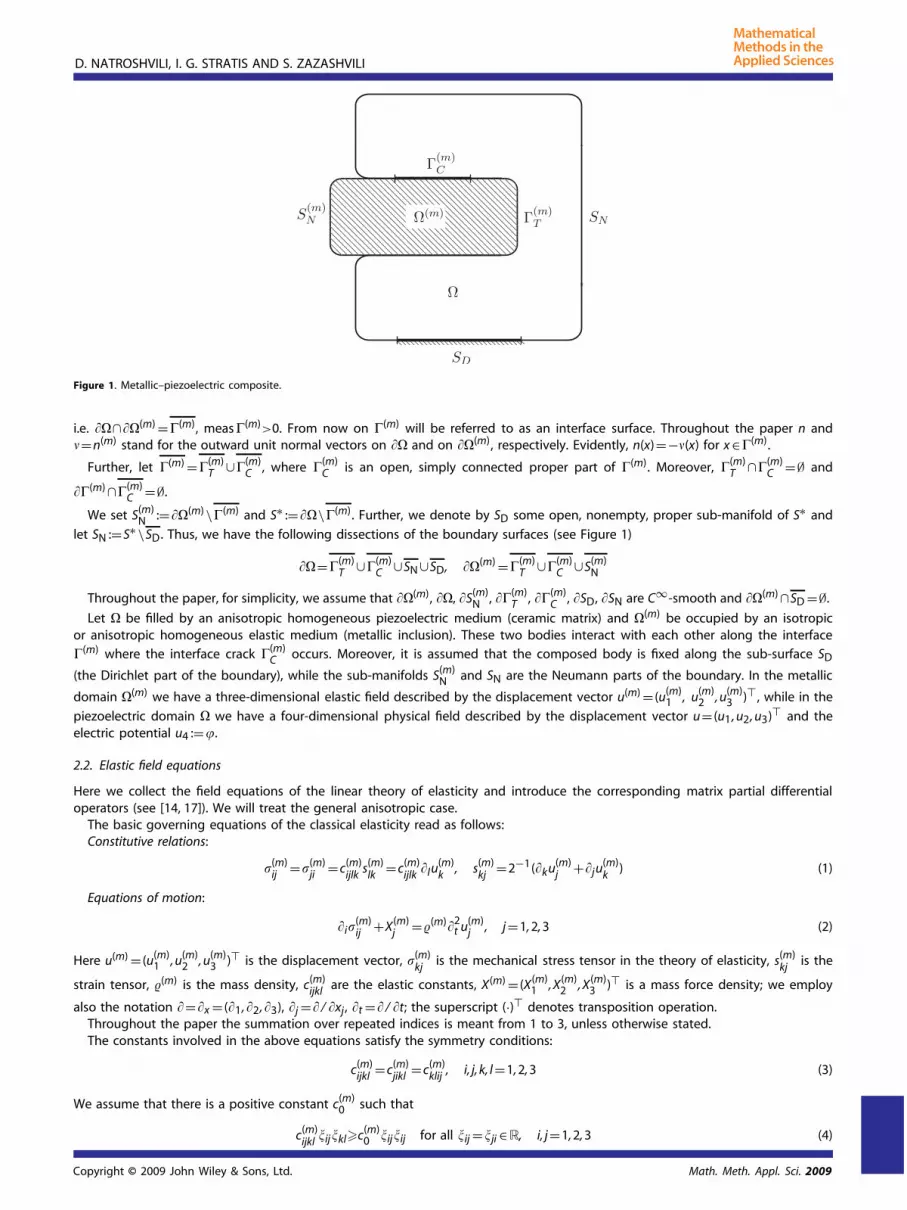
Let �(m) and � be bounded disjoint domains of the three-dimensional Euclidean space R3 with C∞-smooth boundaries ��(m)
and ��, respectively. Moreover, let �� and ��(m) have a nonempty, simply connected intersection �(m) with a positive measure,
i.e. ��∩��(m) =�(m), meas�(m)>0. From now on �(m) will be referred to as an interface surface. Throughout the paper n and�=n(m) stand for the outward unit normal vectors on �� and on ��(m), respectively. Evidently, n(x)=−�(x) for x ∈�(m).
Further, let �(m) =�(m)T ∪�(m)
C , where �(m)C is an open, simply connected proper part of �(m). Moreover, �(m)
T ∩�(m)C =∅ and
��(m) ∩�(m)C =∅.
We set S(m)N :=��(m) \�(m) and S∗ :=��\�(m). Further, we denote by SD some open, nonempty, proper sub-manifold of S∗ and
let SN :=S∗ \SD. Thus, we have the following dissections of the boundary surfaces (see Figure 1)
��=�(m)T ∪�(m)
C ∪SN ∪SD, ��(m) =�(m)T ∪�(m)
C ∪S(m)N
Throughout the paper, for simplicity, we assume that ��(m), ��, �S(m)N , ��(m)
T , ��(m)C , �SD, �SN are C∞-smooth and ��(m) ∩SD =∅.
Let � be filled by an anisotropic homogeneous piezoelectric medium (ceramic matrix) and �(m) be occupied by an isotropicor anisotropic homogeneous elastic medium (metallic inclusion). These two bodies interact with each other along the interface
�(m) where the interface crack �(m)C occurs. Moreover, it is assumed that the composed body is fixed along the sub-surface SD
(the Dirichlet part of the boundary), while the sub-manifolds S(m)N and SN are the Neumann parts of the boundary. In the metallic
domain �(m) we have a three-dimensional elastic field described by the displacement vector u(m) = (u(m)1 , u(m)
2 , u(m)3 )� , while in the
piezoelectric domain � we have a four-dimensional physical field described by the displacement vector u= (u1 , u2, u3)� and theelectric potential u4 :=�.
2.2. Elastic field equations
Here we collect the field equations of the linear theory of elasticity and introduce the corresponding matrix partial differentialoperators (see [14, 17]). We will treat the general anisotropic case.
The basic governing equations of the classical elasticity read as follows:Constitutive relations:
(m)ij =(m)
ji =c(m)ijlk s(m)
lk =c(m)ijlk �lu(m)
k , s(m)kj =2−1(�ku(m)
j +�ju(m)k ) (1)
Equations of motion:
�i(m)ij +X(m)
j =(m)�2t u(m)
j , j =1, 2, 3 (2)
Here u(m) = (u(m)1 , u(m)
2 , u(m)3 )� is the displacement vector, (m)
kj is the mechanical stress tensor in the theory of elasticity, s(m)kj is the
strain tensor, (m) is the mass density, c(m)ijkl are the elastic constants, X(m) = (X(m)
1 , X(m)2 , X(m)
3 )� is a mass force density; we employ
also the notation �=�x = (�1,�2,�3), �j =� / �xj , �t =� / �t; the superscript (·)� denotes transposition operation.Throughout the paper the summation over repeated indices is meant from 1 to 3, unless otherwise stated.The constants involved in the above equations satisfy the symmetry conditions:
c(m)ijkl =c(m)
jikl =c(m)klij , i, j, k, l =1, 2, 3 (3)
We assume that there is a positive constant c(m)0 such that
In particular, this inequality implies that the density of the potential energy corresponding to the displacement vector u(m) ,
E(m)(u(m), u(m))=c(m)ijlk s(m)
ij s(m)lk
is positive definite with respect to the symmetric components of the strain tensor s(m)lk .
Substituting (1) into (2) leads to the equation:
c(m)ijlk �i�lu
(m)k +X(m)
j =(m)�2t u(m)
j , j =1, 2, 3 (5)
The simultaneous Equations (5) represent the basic system of dynamics of the theory of elasticity. If the time dependence of all thefunctions involved in these equations is harmonic, that is if they can be represented as a product of a function of the spatial variables(x1, x2, x3) and of the multiplier exp{�t}, where �=+ i is a complex parameter, we have the pseudo-oscillation equations of thetheory of elasticity. Note that the pseudo–oscillation equations can be obtained from the corresponding dynamical equations bythe Laplace transform. If �= i is a pure imaginary number, with the so-called frequency parameter ∈R, we obtain the steady-stateoscillation equations. Finally, if �=0 we get the equations of statics.
In this paper we will mainly consider the system of pseudo-oscillations
c(m)ijlk �i�lu(m)
k −(m)�2u(m)j +X(m)
j =0, j =1, 2, 3 (6)
In matrix form these equations can be rewritten as
A(m)(�,�)u(m)(x)+X(m)(x)=0
where
A(m)(�,�)= [A(m)jk (�,�)]3×3 , A(m)
jk (�,�)=c(m)ijlk �i�l −(m)�2�jk (7)
Here �jk is the Kronecker delta.
Denote by A(m,0)(�) the principal homogeneous part of the operator (7),
A(m,0)(�)= [c(m)ijlk �i�l]3×3 (8)
By A(m)∗(�,�) we denote the 3×3 matrix differential operator formally adjoint to A(m)(�,�), that is A(m)∗(�,�) := [A(m) (−�,�)]�, wherethe overbar denotes complex conjugation.
With the help of the symmetry conditions (3) and the inequality (4) it can easily be shown that A(m,0)(�) is a formally selfadjointelliptic operator with a positive-definite principal homogeneous symbol matrix, that is,
A(m,0)(�)�·��c(m)|�|2|�|2 for all �∈R3 and for all �∈C3
with some positive constant c(m)>0 depending on the material parameters.Here and in what follows, for two complex–valued vectors a, b∈CN by a·b we denote the scalar product, a·b=∑N
j=1 ajbj .
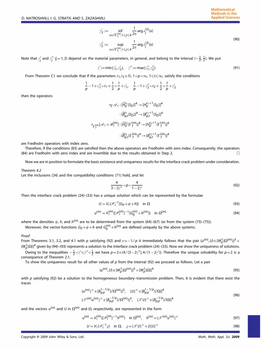
The components of the mechanical stress vector acting on a surface element with a normal �= (�1,�2,�3) are calculated by theformulae
(m)ij �i =c(m)
ijlk �i�lu(m)k , j =1, 2, 3
We introduce the stress operator
T(m)(�,�)= [T(m)jk (�,�)]3×3 , T(m)
jk (�,�)=c(m)ijlk �i�l , j, k =1, 2, 3 (9)
The stress vector associated with the displacement vector u(m) then reads
T(m)u(m) = ((m)i1 �i ,
(m)i2 �i ,(m)
i3 �i)� (10)
2.3. Piezoelastic field equations
In this subsection we collect the field equations of the linear theory of piezoelasticity for a general anisotropic case and introducethe corresponding matrix partial differential operators (cf. [10, 15]).
In piezoelasticity we have the following governing equations:Constitutive relations:
ij = ji =cijkl skl −elijEl =cijkl�luk +elij�l� (11)
Here u= (u1 , u2, u3)� is the displacement vector, � is the electric potential, kj is the mechanical stress tensor in the theory of
electroelasticity, skj is the strain tensor, D is the electric displacement vector, E = (E1, E2, E3)� :=−grad� is the electric field vector, is the mass density, cijkl are the elastic constants, ekij are the piezoelectric constants, �kj are the dielectric (permittivity) constants,
X = (X1, X2, X3)� is a mass force density, X4 is a charge density.From the relations (11)–(14) we derive the linear system of pseudo-oscillation equations of the theory of piezoelasticity:
cijlk�i�luk −�2uj +elij�l�i�+Xj = 0, j =1, 2, 3
−eikl�i�luk +�il�i�l�+X4 = 0(15)
or in matrix form
A(�,�)U(x)+X̃ (x)=0 in � (16)
where U := (u1 , u2, u3, u4)� = (u,�)� and X̃ = (X, X4)� = (X1, X2, X3, X4)�, A(�,�) is the matrix differential operator generated byEquations (15)
Denote by A(0)(�) the principal homogeneous part of the operator (17),
A(0)(�)=[
[cijlk�i�l]3×3 [elij�l�i]3×1
[−eikl�i�l]1×3 �il�i�l
]4×4
(18)
The constants involved in these equations satisfy the symmetry conditions (see, e.g. [15]):
cijkl =cjikl =cklij , eijk =eikj , �ij =�ji , i, j, k, l =1, 2, 3
Moreover, from physical considerations it follows that:
cijkl�ij�kl � c0�ij�ij for all �ij =�ji ∈R (19)
�ij�i�j � c1|�|2 for all �= (�1,�2,�3)∈R3 (20)
where c0 and c1 are positive constants.
By A∗(�,�) := [A(−�,�)]� we denote the operator formally adjoint to A(�,�).With the help of the inequalities (19) and (20), it can easily be shown that the principal part of the operator A(�,�) is formally
nonselfadjoint but strongly elliptic,
A(0)(�)� ·��c|�|2|�|2 for all �∈R3 for all �∈C4
with some positive constant c>0 depending on the material parameters.In the theory of thermopiezoelasticity the components of the three-dimensional mechanical stress vector acting on a surface
element with a normal n= (n1, n2, n3) have the form
ijni =cijlk ni�luk +elij ni�l� for j =1, 2, 3
while the normal component of the electric displacement vector (with opposite sign) reads as
−Dini =−eikl ni�luk +�il ni�l�
Let us introduce the following matrix differential operator:
Clearly, the components of the vector TU given by (23) have the following physical sense: the first three components correspondto the mechanical stress vector in the theory of electroelasticity, and the fourth one is the normal component of the electricdisplacement vector (with opposite sign), respectively.
The following boundary operator, associated with the differential operator A∗(�,�), appears also in Green’s formulae
Let us consider the metallic–piezoelectric composite structure described in Section 2.1 (see Figure 1). We assume that
1. The composed body is fixed along the sub-surface SD, i.e. there are given homogeneous Dirichlet data for the vector U= (u,�)� .
2. The sub-surface S(m)N is traction-free, i.e. the mechanical stress vector T(m)u(m) equals to zero on S(m)
N .3. The sub-surface SN is traction- and charge-free, i.e. the vector TU equals to zero on SN.
4. Along the transmission interface submanifold �(m)T the piezoelectric and metallic solids are bonded, i.e. the rigid contact
conditions are fulfilled, which means that the displacement and mechanical stress vectors are continuous across �(m)T ; moreover,
for the electric potential function � the Dirichlet condition is given on �(m)T due to the rigid contact conditions.
5. The faces of the interface crack �(m)C are traction- and charge-free i.e. the vectors T(m)u(m) and TU equal to zero on �(m)
C .
Solutions to this kind of crack and mixed boundary value problems and related mechanical and electrical characteristics usually
have singularities in a neighbourhood of exceptional curves, ��(m)C , �SD, ��(m). Our goal is to study the solvability of the above
transmission problem in appropriate function spaces and analyse the regularity properties of the solutions. In particular, we describethe dependence of the stress singularity exponents on the material parameters. As we will see below, this dependence is quitenontrivial.
Let us introduce some notation. Throughout the paper the symbol {·}+ denotes the interior one-sided limit on �� (respectively��(m)) from � (respectively �(m)). Similarly, {·}− denotes the exterior one-sided limit on �� (respectively ��(m)) from the exteriorof � (respectively �(m)). We will use also the notation {·}±
��and {·}±
��(m) for the trace operators on �� and ��(m).
By Lp, Wrp, Hs
p, and Bsp,q (with r�0, s∈R, 1<p<∞, 1�q�∞) we denote the well-known Lebesgue, Sobolev–Slobodetski, Bessel
potential, and Besov function spaces, respectively (see, e.g. [22, 23]). Recall that Hr2 =Wr
2 =Br2,2, Hs
2 =Bs2,2, Wt
p =Btp,p , and Hk
p =Wkp ,
for any r�0, for any s∈R, for any positive and noninteger t, and for any nonnegative integer k.Let M0 be a smooth surface without boundary. For a smooth sub-manifold M⊂M0 we denote by H̃s
p(M) and B̃sp,q(M) the
subspaces of Hsp(M0) and Bs
p,q(M0), respectively,
H̃sp(M) = {g : g∈Hs
p(M0), suppg⊂M}
B̃sp,q(M) = {g : g∈Bs
p,q(M0), suppg⊂M}
while Hsp(M) and Bs
p,q(M) denote the spaces of restrictions on M of functions from Hsp(M0) and Bs
p,q(M0), respectively,
Hsp(M) = {rMf : f ∈Hs
p(M0)}
Bsp,q(M) = {rMf : f ∈Bs
p,q(M0)}
where rM is the restriction operator on M.In the sequel, without loss of generality, we shall assume that the mass force densities and the charge density vanish in the
corresponding regions, that is,
X(m)k =0 in �(m) for k =1, 3, Xj =0 in � for j =1, 4
If not, we can write particular solutions to the nonhomogeneous differential equations (6) and (15) explicitly in the form of volumeNewtonian potentials:
u(m)0 (x) = N(m)
�(m) (X(m)) :=−∫�(m)
�(m)(x−y,�)X(m)(y)dy, x ∈�(m)
U0(x) = N�(X) :=−∫�
�(x−y,�)X(y)dy, x ∈�
where �(m)(x−y,�) and �(x−y,�) are fundamental solution matrices of the operators A(m)(�,�) and A(�,�), respectively
(see Appendix B). Note that for X(m)j ∈Lp(�(m)), j =1, 2, 3, and Xk ∈Lp(�), k =1, 2, 3, 4, we have u(m)
0 ∈ [W2p (�(m))]3 and U0 ∈ [W2
p (�)]4.
Therefore, without loss of generality, in what follows we will consider the homogeneous versions of the differential Equations (6)and (15). However, we have to take into consideration that the homogeneous boundary and transmission conditions described initems (1)–(5), above, become then nonhomogeneous.
Now we are in position to formulate mathematically the above interface crack problem:
Problem (ICP): Find vector–functions u(m) = (u(m)1 , u(m)
2 , u(m)3 )� :�(m) →C3 and U= (u1 , u2, u3, u4)� :�→C4 belonging to the spaces
[W1p (�(m))]3 and [W1
p (�)]4 with 1<p<∞, respectively, and satisfying
(i) The systems of partial differential equations:
j and Q(m)j (j =1, 2, 3, 4) have to satisfy some evident compatibility conditions (see Section 4.1,
inclusion (71)). We set
Q = (Q1, Q2, Q3, Q4)� ∈ [B−1/ pp,p (SN)]4
Q̃ = (̃Q1, Q̃2, Q̃3, Q̃4)� ∈ [B−1/ pp,p (�(m)
C )]4
Q(m) = (Q(m)1 , Q(m)
2 , Q(m)3 )� ∈ [B−1/ p
p,p (S(m)N )]3
Q̃(m) = (̃Q(m)1 , Q̃(m)
2 , Q̃(m)3 )� ∈ [B−1/ p
p,p (�(m)C )]3
f = (f1, f2, f3, f4)� ∈ [B1/ p′p,p (SD)]4
f (m) = (f (m)1 , f (m)
2 , f (m)3 , f (m)
4 )� ∈ [B1/ p′p,p (�(m)
T )]4
F(m) = (F(m)1 , F(m)
2 , F(m)3 )� ∈ [B−1/ p
p,p (�(m)T )]3
(35)
A pair (u(m), U)∈ [W1p (�(m))]3 × [W1
p (�)]4 will be called a solution to the boundary–transmission problem (24)–(33).
The differential Equations (24) and (25) are understood in the distributional sense, in general. We remark that if u(m) ∈ [W1p (�(m))]3
and U∈ [W1p (�)]4 solve the homogeneous differential equations then actually we have the inclusions u(m) ∈ [C∞(�(m))]3 and
U∈ [C∞(�)]4 due to the ellipticity of the corresponding differential operators. In fact, u(m) and U are complex-valued analytic vectorsof spatial real variables (x1, x2, x3) in �(m) and �, respectively.
The Dirichlet-type conditions (28), (29), and (30) involving boundary limiting values of the vectors u(m) and U are understoodin the usual trace sense, while the Neumann-type conditions (26), (27), (31), (32) and (33) involving boundary limiting values ofthe vectors T(m)u(m) and TU are understood in the functional sense defined by the relations related to Green’s formulae (seeAppendix A, formulae (A2) and (A4))
p′ (�(m))]3 and V = (v, v4)� ∈ [W1p′ (�)]4 are arbitrary vector-functions with v = (v1, v2, v3)� , E(u, v)=
cijlk�iuj�lvk and E(m)(u(m), v(m))=c(m)ijlk �iu(m)
j �lv(m)k . Here 〈·, ·〉��(m) (respectively 〈·, ·〉��) denotes the duality between the function
spaces [B−1/ pp,p (��(m))]3 and [B1/ p
p′,p′ (��(m))]3 (respectively [B−1/ pp,p (��)]4 and [B1/ p
p′ ,p′ (��)]4) which extends the usual L2 scalar product
〈f, g〉M=∫M
N∑j=1
fjgj dM for f, g∈ [L2(M)]N, M∈{��(m),��}
By standard arguments it can easily be shown that the ‘generalized traces’, i.e. the functionals
{T(m)(�,�)u(m)}+ ∈ [B−1/ pp,p (��(m))]3 and {T(�, n)U}+ ∈ [B−1/ p
p,p (��)]4
are correctly determined by the above relations, provided that A(m)(�,�)u(m) ∈ [Lp(�(m))]3 and A(�,�)U∈ [Lp(�)]4.Now, we prove the following uniqueness theorem for p=2. The similar uniqueness theorem for p �=2 will be proved later in
Section 4 (see Theorem 4.2).
Theorem 2.1Let �=+ i and either �=0 or �=0. The homogeneous boundary–transmission problem (24)–(33) has only the trivial solution inthe space [W1
2 (�(m))]3 × [W12 (�)]4, provided meas SD>0.
ProofLet a pair (u(m) , U)∈ [W1
2 (�(m))]3 × [W12 (�)]4 be a solution to the homogeneous boundary–transmission problem (24)–(33). Green’s
formulae (36) with v(m) =u(m) and∫�
[3∑
j=1[AU]juj +[AU]4u4
]dx =−
∫�
[E(u, u)+�2|u|2 +�jl�lu4�ju4]dx+3∑
j=1〈{TU}+j ,{uj}+〉��+〈{TU}+4 ,{u4}+〉�� (38)
along with the homogeneous boundary and transmission conditions then imply∫�(m)
Note that due to the relations (4), (19) and (20), we have
E(m)(u(m), u(m))�0, E(u, u)�0, �jl�lu4�ju4�0 (40)
with the equality holding only for complex rigid displacement vectors and a constant potential field,
u(m) =a(m) ×x+b(m), u=a×x+b, u4 =a4 (41)
where a(m), b(m), a, b∈C3, a4 ∈C, and × denotes the usual cross product of two vectors.Taking into account the above inequalities and separating the real and imaginary parts of (39) we obtain∫
�(m)[E(m)(u(m) , u(m))+(m)(2 − 2)|u(m)|2]dx+
∫�
[E(u, u)+(2 − 2)|u|2 +�jl�lu4�ju4]dx = 0 (42)
∫�(m)
2(m) |u(m)|2 dx+∫�
2 |u|2 dx = 0 (43)
First, let us assume that �=0 and �=0. With the help of the homogeneous boundary and transmission conditions we easily
derive from (43) that u(m)j =0, j =1, 3 in �(m) and uj =0, j =1, 3 in �. From (42) we then conclude that u4 =0 in � due to (40) and
the homogeneous Dirichlet boundary conditions on SD ∪�(m)T . Thus u(m) =0 in �(m) and U=0 in �.
The proof for the cases �=0 and =0, or �=0 can be performed verbatim. �
Below we apply the potential method to study the existence of solutions in different function spaces and to establish theirregularity properties.
3. Layer potentials
Here, we present basic properties of the layer potentials and certain boundary integral (pseudodifferential) operators generated bythem. These results are crucial in our analysis.
3.1. Layer potentials
Let �(m)(·,�)= [�(m)kj (·,�)]3×3 and �(·,�)= [�kj(·,�)]4×4 be the fundamental matrix–functions of the differential operators A(m)(�x,�)
and A(�x,�) (see Appendix B), and introduce the single and double layer potentials:
V (m)� (h(m))(x) =
∫��(m)
�(m)(x−y,�) h(m)(y)dy S
W(m)� (h(m))(x) =
∫��(m)
[T(m)(�y,�(y))�(m)(x−y,�)]�h(m)(y)dy S
V�(h)(x) =∫��
�(x−y,�)h(y)dy S
W�(h)(x) =∫��
[T̃(�y, n(y))[�(x−y,�)]�]�h(y)dy S
where h(m) = (h(m)1 , h(m)
2 , h(m)3 )� and h= (h1 , h2, h3, h4)� are densities of the potentials. For the readers’ convenience, here we collect
some results concerning these layer potentials and the corresponding boundary operators needed in subsequent analysis. We recallthat ��, ��(m) ∈C∞, while n and � are outward normals to �� and ��(m), respectively.
Theorem 3.1Let 1<p<∞, 1�t�∞, and s∈R. The operators
ProofFor regular densities the proof for the potentials V (m)
� and W(m)� can be found in [14], in the isotropic case, and in [21, 24, 25], in the
anisotropic case, while for the potentials V� and W� the proof is given in [26, 27] (see also [12]).Note that the main ideas for generalization to the scale of Bessel potential spaces and Besov spaces are based on the duality
and interpolation technique that is described in [28], in view of the theory of pseudodifferential operators on smooth manifoldswithout boundary (see also [29, 30]). �
For the boundary integral (pseudodifferential) operators generated by the layer potentials we will employ the following notation:
H(m)� (h(m))(x) :=
∫��(m)
�(m)(x−y,�)h(m)(y)dy S
K(m)� (h(m))(x) :=
∫��(m)
[T(m)(�x,�(x))�(m)(x−y,�)]h(m)(y)dy S
K̃(m)∗� (h(m))(x) :=
∫��(m)
[T(m)(�y,�(y))�(m)(x−y,�)]�h(m)(y)dy S
H�(h)(x) :=∫��
�(x−y,�)h(y)dy S
K�(h)(x) :=∫��
[T(�x, n(x))�(x−y,�)]h(y)dy S
K̃∗� (h)(x) :=
∫��
[T̃(�y, n(y))[�(x−y,�)]�]�h(y)dy S
L(m)� (h(m))(x) := {T(m)(�x,�(x))W(m)(h(m))(x)}±
L�(h)(x) := {T(�x, n(x))W�(h)(x)}±
The layer boundary operators H(m)� , H� and L(m)
� , L� are pseudodifferential operators of order −1 and 1, respectively, while
the operators K(m)� , K̃
(m)∗� , K� and K̃
∗� are singular integral operators, i.e. pseudodifferential operators of order 0 (for details see
3.2. Auxiliary problems and representation formulae of solutions
Here we assume that �= �=0 and consider two auxiliary boundary value problems needed for our further analysis.
3.2.1. Auxiliary problem I. Find a vector u(m) = (u(m)1 , u(m)
2 , u(m)3 )� :�(m) →C3 which belongs to the space [W1
2 (�(m))]3 and satisfiesthe following conditions:
A(m)(�,�)u(m) = 0 in �(m) (44)
{T(m)u(m)}+ = �(m) on ��(m) (45)
where �(m) = (�(m)1 ,�(m)
2 ,�(m)3 )� ∈ [H−1/ 2
2 (��(m))]3. With the help of Green’s formula it can easily be shown that the homogeneousversion of this auxiliary BVP possesses only the trivial solution.
From Theorem 3.4 and the uniqueness result for the BVP (44)–(45) immediately follows
Lemma 3.5Let �= �=0 and 1<p<∞. An arbitrary solution u(m) ∈ [W1
p (�(m))]3 to the homogeneous Equation (44) can be uniquely representedby the single layer potential
u(m)(x)=V (m)� ([P(m)
� ]−1�(m))(x), x ∈�(m) (46)
where
P(m)� :=−2−1 I3 +K(m)
� , �(m) ={T(m)u(m)}+ ∈ [B−1/ pp,p (��(m))]3 (47)
ProofEvidently, if �(m) = (�(m)
1 ,�(m)2 ,�(m)
3 )� ∈ [B−1/ pp,p (��(m))]3 then the vector (47) solves the auxiliary BVP and belongs to the space
[W1p (�(m))]3 by Theorem 3.1. The uniqueness follows from the general integral representation formula (B5) and Theorem 3.4. �
3.2.2. Auxiliary problem II. Find a vector-function U= (u1 , u2, u3, u4)� :�→C4 which belongs to the space [W12 (�)]4 and satisfies the
following conditions:
A(�,�)U = 0 in � (48)
{TU}++�{U}+ = � on �� (49)
where � := (�1,�2,�3,�4)� ∈ [H−1/ 22 (��)]4, � is a smooth real-valued scalar function which does not vanish identically and
��0, supp�⊂SD (50)
By the same arguments as in the proof of Theorem 2.1 we can easily show that the homogeneous version of this boundary valueproblem possesses only the trivial solution in [W1
2 (�)]4.
We look for a solution to the Auxiliary Problem II in the form of a single layer potential, U(x)=V�(f )(x), where f = (f1, f2, f3, f4)� ∈[H−1/ 2
2 (��)]4 is a sought density. The boundary condition (49) leads then to the system of equations:
(−2−1 I4 +K�)f +�H�f =� on ��
Denote the matrix operator generated by the left-hand side expression of this equation by P� and rewrite the system as
ProofFrom the uniqueness result for the Auxiliary Problem II it follows that the operator (52) is injective for p=2 and s=− 1
2 . The operator
H� : [H−1/ 22 (��)]4 → [H−1/ 2
2 (��)]4 is compact. By Theorem 3.4 we then conclude that the index of the operator (52) equals to zero.Since P� is an injective singular integral operator of normal type with zero index it follows that it is surjective. Thus, the operator(52) is invertible for p=2 and s=− 1
2 .The invertibility of the operators (52) and (53) for all 1<p<∞, 1�t�∞, and s∈R then follows by standard duality and interpolation
arguments for the C∞-regular surface �� (see, e.g. [32, 28]). �
As a consequence we have the following representation formula.
Lemma 3.7Let �= �=0 and 1<p<∞. An arbitrary solution U∈ [W1
p (�)]4 to the homogeneous Equation (48) can be uniquely represented by
the single layer potential U(x)=V�(P−1� �)(x), where �={TU}++�{U}+ ∈ [B−1/ p
p,p (��)]4.
4. Existence and regularity results
4.1. Reduction to boundary equations
Let us return to the interface crack problem (24)–(33) and derive the equivalent boundary integral formulation of this problem.Keeping in mind (35), let
G :=⎧⎨⎩Q on SN,
Q̃ on �(m)C ,
G(m) :=⎧⎨⎩Q(m) on S(m)
N
Q̃(m) on �(m)C
G ∈ [B−1/ pp,p (SN ∪�(m)
C )]4, G(m) ∈ [B−1/ pp,p (S(m)
N ∪�(m)C )]3
(54)
and
G0 = (G01,. . . , G04)� ∈ [B−1/ pp,p (��)]4
G(m)0 = (G(m)
01 ,. . . , G(m)03 )� ∈ [B−1/ p
p,p (��(m))]3
be some fixed extensions of the vector-function G and G(m), respectively, onto �� and ��(m) preserving the space. It is evident thatarbitrary extensions of the same vector-functions can be represented then as
G∗ =G0 +�+h, G(m)∗ =G(m)0 +h(m) (55)
where
� = (�1,. . . ,�4)� ∈ [̃B−1/ pp,p (SD)]4
h = (h1,. . . , h4)� ∈ [̃B−1/ pp,p (�(m)
T )]4 (56)
h(m) = (h(m)1 , h(m)
2 , h(m)3 )� ∈ [̃B−1/ p
p,p (�(m)T )]3 (57)
are arbitrary vector-functions.We develop here the indirect boundary integral equations method. In accordance with Lemmata 3.5 and 3.7 we look for a solution
pair (u(m) , U) of the interface crack problem (24)–(33) in the form of single layer potentials,
u(m) = (u(m) ,. . . , u(m)3 )� =V (m)
� ([P(m)� ]−1[G(m)
0 +h(m)]) in �(m) (58)
U = (u1,. . . , u4)� =V�(P−1� [G0 +�+h]) in � (59)
where P(m)� and P� are given by (47) and (51), and h(m), h and � are unknown vector-functions satisfying the inclusions (56) and (57).
By Lemmata 3.5 and 3.7 we see that the homogeneous differential Equations (24)–(25), the boundary conditions (26)–(27) andcrack conditions (32)–(33) are satisfied automatically.
The remaining boundary and transmission conditions (28)–(31) lead to the equations
rSD [H�P−1� [G0 +�+h]]k = fk on SD, k =1, 4 (60)
r�(m)T
[H�P−1� [G0 +�+h]]4 = f (m)
4 on �(m)T (61)
r�(m)T
[H�P−1� [G0 +�+h]]j −r�(m)
T[H(m)
� [P(m)� ]−1[G(m)
0 +h(m)]]j = f (m)j on �(m)
T , j =1, 3 (62)
r�(m)T
[G0 +�+h]j +r�(m)T
[G(m)0 +h(m)]j = F(m)
j on �(m)T , j =1, 3 (63)
Finally, we arrive at the simultaneous pseudodifferential equations with respect to the unknown vector-functions �, h and h(m)
rSD[H�P
−1� [�+h]]k = f̃k on SD, k =1, 4 (64)
r�(m)T
[H�P−1� [�+h]]4 = f̃ (m)
4 on �(m)T (65)
r�(m)T
[H�P−1� [�+h]]j −r�(m)
T[H(m)
� [P(m)� ]−1[h(m)]]j = f̃ (m)
j on �(m)T , j =1, 3 (66)
r�(m)T
h(m)j +r�(m)
Thj = F̃(m)
j on �(m)T , j =1, 3 (67)
where
f̃k := fk −rSD [H�P−1� G0]k ∈B1−1/ p
p,p (SD), k =1, 4 (68)
f̃ (m)4 := f (m)
4 −r�(m)T
[H�P−1� G0]4 ∈B1−1/ p
p,p (�(m)T ) (69)
f̃ (m)j := f (m)
j +r�(m) [H(m)� [P(m)
� ]−1G(m)0 ]j −r�(m) [H�P
−1� G0]j ∈B1−1/ p
p,p (�(m)), j =1, 3 (70)
F̃(m)j := F(m)
j −r�(m)T
G0j −r�(m)T
G(m)0j ∈ r�(m)
TB̃−1/ p
p,p (�(m)T ), j =1, 3 (71)
The last inclusions are the compatibility conditions for Problem (ICP). Therefore, in what follows we assume that F̃(m)j is extended
It is easy to see that the simultaneous Equations (60)–(63) and (73)–(75), where the right-hand sides are related by the equalities(68)–(71) and (76)–(78), are equivalent in the following sense: if the triplet
(�, h, h(m))∈ [̃B−1/ pp,p (SD)]4 × [̃B−1/ p
p,p (�(m)T )]4 × [̃B−1/ p
p,p (�(m)T )]3
solves the system (73)–(75), then the pair (G0 +�+h, G(m)0 +h(m)) solves the system (60)–(63), and vice versa.
4.2. Existence theorems and regularity of solutions
Here we show that the system of pseudodifferential Equations (73)–(75) is uniquely solvable in appropriate function spaces. To thisend, let us put
N� :=
⎡⎢⎢⎢⎢⎣rSDA� rSDA� rSD [0]4×3
r�(m)T
A� r�(m)T
[A�+B(m)� ] r�(m)
T[0]4×3
r�(m)T
[0]3×4 r�(m)T
I3×4 r�(m)T
I3
⎤⎥⎥⎥⎥⎦11×11
(80)
with
I3×4 :=
⎡⎢⎢⎣1 0 0 0
0 1 0 0
0 0 1 0
⎤⎥⎥⎦Further, let
� := (�, h, h(m))�, Y := (̃f , g̃(m), F̃(m))�
Xsp := [̃Bs
p,p(SD)]4 × [̃Bsp,p(�(m)
T )]4 × [̃Bsp,p(�(m)
T )]3
Ysp := [Bs+1
p,p (SD)]4 × [Bs+1p,p (�(m)
T )]4 × [̃Bsp,p(�(m)
T )]3
Xsp,t := [̃Bs
p,t(SD)]4 × [̃Bsp,t(�(m)
T )]4 × [̃Bsp,t(�(m)
T )]3
Ysp,t := [Bs+1
p,t (SD)]4 × [Bs+1p,t (�(m)
T )]4 × [̃Bsp,t(�(m)
T )]3
We have the following mapping properties
N� :Xsp →Ys
p [Xsp,t →Ys
p,t] (81)
for s∈R, 1<p<∞ and 1�t�∞, due to Theorems 3.3, 3.4 and Lemma 3.6.Evidently, we can rewrite the system (73)–(75) as
N��=Y (82)
where �∈Xsp is the above introduced unknown vector and Y ∈Ys
p is a given vector.As we will see below the operator (81) is not invertible for all s∈R. The interval of invertibility a<s<b depends on p and on
some parameters �′ and �′′ which are determined by the eigenvalues of special matrices constructed by means of the principal
homogeneous symbol matrices of the operators A� and A�+B(m)� (see (72) and (91)). Note that the numbers �′ and �′′ define
also Hölder smoothness exponents for the solutions to the original interface crack problem in a neighbourhood of the exceptional
curves �SD, ��(m)C and ��(m).
We start with the following theorem.
Theorem 4.1Let the conditions
1<p<∞, 1�t�∞,1
p−1+�′′<s+ 1
2<
1
p+�′ (83)
be satisfied with �′ and �′′ given by (89), (90), and (91). Then the operators
N� :Xsp →Ys
p [Xsp,t →Ys
p,t] (84)
are invertible.
ProofWe prove the theorem in several steps. First, we show that the operators (84) are Fredholm with zero index and afterwards weestablish that the corresponding null–spaces are trivial.
Step 1: First of all let us remark that the operators
are compact since SD ∪�(m)T =∅. Further we establish that the operators
rSDA� : [̃H−1/ 22 (SD)]4 → [H1/ 2
2 (SD)]4
r�(m)T
[A�+B(m)� ] : [̃H−1/ 2
2 (�(m)T )]4 → [H1/ 2
2 (�(m)T )]4
(86)
are strongly elliptic, Fredholm pseudodifferential operators of order −1 with index zero. We remark that the principal homogeneoussymbol matrices of these operators are strongly elliptic (see Appendix B).
Using Green’s formula (A4) and Korn’s inequality (see, e.g. [33]), for an arbitrary solution vector U∈ [H12(�)]4 ≡ [W1
2 (�)]4 to thehomogeneous equation A(�,�)U=0 in � by standard arguments we get
〈[U]+ , [TU]+〉���c1||U||2[H1
2(�)]4 −c2||U||2[H0
2(�)]4 (87)
Substitute here U=V�(P−1� �) with �∈ [H−1/ 2
2 (��)]4. Owing to the equality �=P�H−1� {U}+ and boundedness of the operators
involved, we have ||�||2[H−1/2
2 (��)]4�c∗||{U}+||2
[H1/22 (��)]4
with some positive constant c∗. Therefore, by the trace theorem from (87)
we easily obtain
〈H�P−1� �,�〉���c′
1||�||2[H−1/2
2 (��)]4 +||�HP−1� �||[H−1/2
2 (��)]4 −c′2||V�(P−1
� �)||2[H0
2(�)]4
In particular, in view of Theorem 3.1 and Lemma 3.6 for all �∈ [̃H−1/ 22 (SD)]4 we have
〈rSDH�P−1� �,�〉���c′′
1||�||2[̃H−1/2
2 (SD)]4 −c′′2 ||�||2
[̃H−3/22 (SD)]4 (88)
From (88) it follows that the operator rSDA� = rSDH�P−1� : [̃H−1/ 2
2 (SD)]4 → [H1/ 22 (SD)]4 is a strongly elliptic pseudodifferential
Fredholm operator with index zero.
Then it follows that the same is true for the operator (86) since the principal homogeneous symbol matrix of the operator B(m)�
is nonnegative (see Appendix B).Therefore, due to the compactness of the operators (85), the operator (84) is Fredholm with index zero for s=− 1
2 , p=2 andt=2.
Step 2: In view of the uniqueness result (Theorem 2.1), via the representation formulae (58) and (59) with G(m)0 =0 and G0 =0, we
can easily show that the operator (84) is injective for s=− 12 , p=2, and t=2. Since its index is zero, we conclude that it is surjective.
Thus the operator (84) is invertible for s=− 12 , p=2, and t=2.
Step 3: To complete the proof for the general case we proceed as follows. We see that the following upper triangular operator:
N(0)� :=
⎡⎢⎢⎢⎢⎣rSD
A� rSD[0]4×4 rSD
[0]4×3
r�(m)T
[0]4×4 r�(m)T
[A�+B(m)� ] r�(m)
T[0]4×3
r�(m)T
[0]3×4 r�(m)T
I3×4 r�(m)T
I3
⎤⎥⎥⎥⎥⎦11×11
is a compact perturbation of the operator (80). Therefore, we have to investigate Fredholm properties of the operators
rSDA� : [̃Bs
p,t(SD]4 → [Bs+1p,t (SD)]4
r�(m)T
[A�+B(m)� ] : [̃Bs
p,t(�(m)T )]4 → [Bs+1
p,t (�(m)T )]4
To this end, we apply the results presented in Appendix B. Let 1(x,�1,�2) :=(A�)(x,�1,�2) be the principal homogeneous symbol
matrix of the operator A� and �(1)j (x) (j =1, 4) be the eigenvalues of the matrix D1(x) := [1(x, 0,+1)]−11(x, 0,−1) for x ∈�SD (see
(B14) and (B15)).Similarly, let 2(x,�1,�2)=(A�+B(m)
� )(x,�1,�2) be the principal homogeneous symbol matrix of the operator A�+B(m)� and
�(2)j (x) (j =1, 4) be the eigenvalues of the corresponding matrix D2(x) := [2(x, 0,+1)]−12(x, 0,−1) for x ∈��(m)
T (see (B14) and (B15)).
Note that the curve ��(m)T is the union of the curves where the interface intersects the exterior boundary, ��(m), and the crack
Note that �′j and �′′j (j =1, 2) depend on the material parameters, in general, and belong to the interval (− 1
2 , 12 ). We put
�′ :=min{�′1,�′2}, �′′ :=max{�′′1 ,�′′
2} (91)
From Theorem C1 we conclude that if the parameters r1, r2 ∈R, 1<p<∞, 1�t�∞, satisfy the conditions
1
p−1+�′′
1<r1 + 1
2<
1
p+�′
1,1
p−1+�′′
2<r2 + 1
2<
1
p+�′
2
then the operators
r�A� : [̃Hr1p (SD)]4 → [Hr1+1
p (SD)]4
: [̃Br1p,t(SD)]4 → [Br1+1
p,t (SD)]4
r�(m)T
[A�+B(m)� ] : [̃Hr2
p (�(m)T )]4 → [Hr2+1
p (�(m)T )]4
: [̃Br2p,t(�(m)
T )]4 → [Br2+1p,t (�(m)
T )]4
are Fredholm operators with index zero.Therefore, if the conditions (83) are satisfied then the above operators are Fredholm with zero index. Consequently, the operators
(84) are Fredholm with zero index and are invertible due to the results obtained in Step 2. �
Now we are in position to formulate the basic existence and uniqueness results for the interface crack problem under consideration.
Theorem 4.2Let the inclusions (34) and the compatibility conditions (71) hold, and let
4
3−2�′′ <p<4
1−2�′ (92)
Then the interface crack problem (24)–(33) has a unique solution which can be represented by the formulae
U = V�(P−1� [G0 +�+h]) in � (93)
u(m) = V (m)� ([P(m)
� ]−1[G(m)0 +h(m)]) in �(m) (94)
where the densities �, h, and h(m) are to be determined from the system (64)–(67) (or from the system (73)–(75)).
Moreover, the vector-functions G0 +�+h and G(m)0 +h(m) are defined uniquely by the above systems.
ProofFrom Theorems 3.1, 3.2, and 4.1 with p satisfying (92) and s=−1 / p it immediately follows that the pair (u(m), U)∈ [W1
p (�(m))]3 ×[W1
p (�)]4 given by (94)–(93) represents a solution to the interface crack problem (24)–(33). Now we show the uniqueness of solutions.
Owing to the inequalities − 12 <�′��′′< 1
2 we have p=2∈ (4 / (3−2�′′), 4 / (1−2�′)). Therefore the unique solvability for p=2 is aconsequence of Theorem 2.1.
To show the uniqueness result for all other values of p from the interval (92) we proceed as follows. Let a pair
(u(m), U)∈ [W1p (�(m))]3 × [W1
p (�)]4 (95)
with p satisfying (92) be a solution to the homogeneous boundary–transmission problem. Then, it is evident that there exist thetraces
{u(m)}+ ∈ [B1−1/ pp,p (��(m))]3, {U}+ ∈ [B1−1/ p
p,p (��)]4
{T(m)u(m)}+ ∈ [B−1/ pp,p (��(m))]3, {TU}+ ∈ [B−1/ p
p,p (��)]4(96)
and the vectors u(m) and U in �(m) and �, respectively, are represented in the form
due to Lemmata 3.5 and 3.7. Moreover, due to the homogeneous boundary and transmission conditions we have �=h+� and
h(m) ∈ [̃B−1/ pp,p (�(m)
T )]3, �∈ [̃B−1/ pp,p (SD)]4, h∈ [̃B−1/ p
p,p (�(m)T )]4 (99)
By the same arguments as above we arrive at the homogeneous system
N��=0 with � := (�, h, h(m))� ∈X−1/ pp
Owing to Theorem 4.1, �=0 and we conclude that u(m) =0 in �(m) and U=0 in �.The last assertion of the theorem is trivial and is an obvious consequence of the fact that if the single layer potentials (93) and
(94) vanish identically in � and �(m), then the corresponding densities vanish as well. �
Finally, we can prove the following regularity result for the solution of Problem (ICP).
Theorem 4.3Let the inclusions (34) and the compatibility conditions (71) hold, 1<r<∞, 1�t�∞, and
4
3−2�′′ <p<4
1−2�′ ,1
r− 1
2+�′′<s<
1
r+ 1
2+�′ (100)
Further, let u(m) ∈ [W1p (�(m))]3 and U∈ [W1
p (�)]4 be a unique solution pair of the interface crack problem (24)–(33). Then the followinghold:
(i) if (for k =1, 4, j =1, 3)
Qk ∈ Bs−1r,r (SN), Q(m)
j ∈Bs−1r,r (S(m)
N ), fk ∈Bsr,r(SD), f (m)
k ∈Bsr,r (�(m)
T )
F(m)j ∈ Bs−1
r,r (�(m)T ), Q̃(m)
j ∈Bs−1r,r (�(m)
C ), Q̃k ∈Bs−1r,r (�(m)
C )
and the compatibility conditions
F̃(m)j :=F(m)
j −r�(m)T
G0j −r�(m)T
G(m)0j ∈ r�(m)
TB̃s−1
r,r (�(m)T ), j =1, 3
are satisfied, then u(m) ∈ [Hs+1/ rr (�(m))]3 and U∈ [Hs+1/ r
r (�)]4
(ii) if (for k =1, 4, j =1, 3)
Qk ∈ Bs−1r,t (SN), Q(m)
j ∈Bs−1r,t (S(m)
N ), fk ∈Bsr,t(SD), f (m)
k ∈Bsr,t(�(m)
T )
F(m)j ∈ Bs−1
r,t (�(m)T ), Q̃(m)
j ∈Bs−1r,t (�(m)
C ), Q̃k ∈Bs−1r,t (�(m)
C )
and the compatibility conditions
F̃(m)j :=F(m)
j −r�(m)T
G0j −r�(m)T
G(m)0j ∈ r�(m)
TB̃s−1
r,t (�(m)T ), j =1, 3
are satisfied, then
u(m) ∈ [Bs+ 1
rr,t (�(m))]3, U∈ [Bs+1/ r
r,t (�)]4 (101)
(iii) if �>0 is not an integer and for k =1, 4, j =1, 3
ProofThe proof of items (i) and (ii) easily follows from Theorems 4.1, 4.2, and 3.1.
To prove (iii) we use the following embedding relations (see, e.g. [23])
C�(M)=B�∞,∞(M)⊂B�−�∞,1(M)⊂B�−�
∞,t (M)⊂B�−�r,t (M)⊂C�−�−k/ r(M) (103)
where � is an arbitrary small positive number, M⊂R3 is a compact k-dimensional (k =2, 3) smooth manifold with smooth boundary,1�t�∞, 1<r<∞, �−�−k / r>0, and � and �−�−k / r are not integers.
From (102) and the embedding (103) the condition (101) follows for any s��−�.Bearing in mind (100) and taking r sufficiently large and � sufficiently small, we can put
s=�−� if1
r− 1
2+�′′<�−�<
1
r+ 1
2+�′ (104)
and
s∈(
1
r− 1
2+�′′, 1
r+ 1
2+�′
)if
1
r+ 1
2+�′<�−� (105)
By (101) for the solution vectors we have u(m) ∈ [Bs+1/ rr,t (�(m))]3 and U∈ [Bs+1/ r
r,t (�)]4 with s+1 / r =�−�+1 / r if (104) holds, and
with s+1 / r ∈ (2 / r−1 / 2+�′′, 2 / r+ 12 +�′) if (105) holds. In the last case we can take s+1 / r =2 / r+1 / 2+�′−�. Therefore, we have
either
u(m) ∈ [B�−�+1/ rr,t (�(m))]3, U∈ [B�−�+1/ r
r,t (�)]4
or
u(m) ∈ [B1/ 2+2/ r+�′−�r,t (�(m))]3, U∈ [B
1/ 2+2/ r+�′−�r,t (�)]4
in accordance with the inequalities (104) and (105). The last embedding in (103) (with k =3) yields then that either
where �=min{�, �′+1 / 2}. Since r is sufficiently large and � is sufficiently small, the inclusions (106) complete the proof. �
4.3. Stress singularity exponents
A more detailed analysis based on the asymptotic expansions of solutions (see [19, 34]) shows that for sufficiently smooth boundarydata (C∞ data, say) the principal dominant singular terms of the solution vectors u(m) and U near the exceptional curves �SD and
��(m)T can be represented as a product of a ‘nice’ vector–function and a singular factor of the form [ln(x)]mj−1[(x)]�j+i�j . Note
that the crack edge ��(m)C is a proper connected part of the curve ��(m)
T . Here (x) is the distance from a reference point x tothe exceptional curves. Therefore, near these curves the dominant singular terms of the corresponding generalized stress vectors
T(m)u(m) and TU are represented as a product of a ‘nice’ vector-function and the factor [ln (x)]mj−1[(x)]−1+�j+i�j . The numbers�j are different from zero, in general, and describe the oscillating character of the stress singularities.
The exponents �j + i�j are related to the corresponding eigenvalues of the matrices (B15) (see Appendix B) by the equalities
�j =1
2+ arg�j
2�, �j =− ln |�j|
2�
Here �j ∈{�(1)1 (x),. . . ,�(1)
4 (x)} for x ∈�SD, and �j ∈{�(2)1 (x),. . . ,�(2)
4 (x)} for x ∈��(m)T . In the above expressions the parameter mj denotes
the multiplicity of the eigenvalue �j . It is evident that at the exceptional curves the components of the generalized stress vector
behave like O([ln(x)]m0−1[(x)]−1/ 2+�′), where m0 denotes the maximal multiplicity of the eigenvalues. This is a global singularity
effect for the first-order derivatives of the vectors u(m) and U. Note that �j , �j , and �′ depend on the material parameters; moreover,
�′ is non–positive and �j �=0, in general. This is related to the fact that the eigenvalues �j are complex and, in general, |�j| �=1 (seeAppendix B).
A specific example: Recall that of the 32 crystal classes, 21 are noncentrosymmetric, and of these, 20 exhibit direct piezoelectricity.For numerical calculations we consider the special cases where the domain �(m) is occupied by the isotropic metallic materialpalladium (Pd)–silver (Ag) alloy, whereas the domain � is occupied by one of the following piezoelectric materials: either BariumTitanate (BaTiO3, with tetragonal crystal structure of class 4mm), which belongs to the group of electrical ceramics and is an oxide
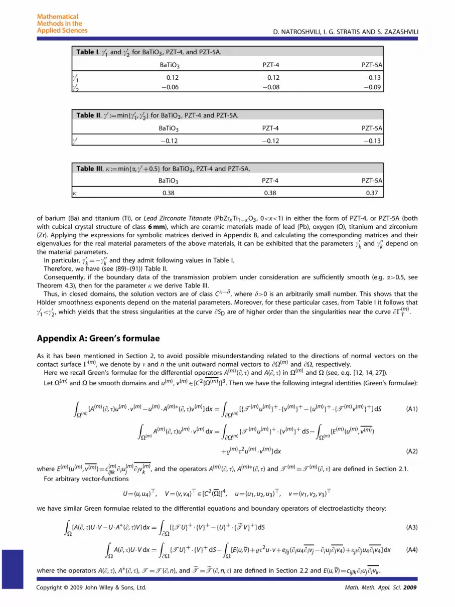
Table III. � :=min{�,�′+0.5} for BaTiO3, PZT-4 and PZT-5A.
BaTiO3 PZT-4 PZT-5A
� 0.38 0.38 0.37
of barium (Ba) and titanium (Ti), or Lead Zirconate Titanate (PbZrxTi1−x O3, 0<x<1) in either the form of PZT-4, or PZT-5A (bothwith cubical crystal structure of class 6 mm), which are ceramic materials made of lead (Pb), oxygen (O), titanium and zirconium(Zr). Applying the expressions for symbolic matrices derived in Appendix B, and calculating the corresponding matrices and theireigenvalues for the real material parameters of the above materials, it can be exhibited that the parameters �′
k and �′′k depend on
the material parameters.In particular, �′
k =−�′′k and they admit following values in Table I.
Therefore, we have (see (89)–(91)) Table II.Consequently, if the boundary data of the transmission problem under consideration are sufficiently smooth (e.g. �>0.5, see
Theorem 4.3), then for the parameter � we derive Table III.Thus, in closed domains, the solution vectors are of class C�−� , where �>0 is an arbitrarily small number. This shows that the
Hölder smoothness exponents depend on the material parameters. Moreover, for these particular cases, from Table I it follows that
�′1<�′2, which yields that the stress singularities at the curve �SD are of higher order than the singularities near the curve ��(m)
T .
Appendix A: Green’s formulae
As it has been mentioned in Section 2, to avoid possible misunderstanding related to the directions of normal vectors on thecontact surface �(m), we denote by � and n the unit outward normal vectors to ��(m) and ��, respectively.
Here we recall Green’s formulae for the differential operators A(m)(�,�) and A(�,�) in �(m) and � (see, e.g. [12, 14, 27]).
Let �(m) and � be smooth domains and u(m), v(m) ∈ [C2(�(m))]3. Then we have the following integral identities (Green’s formulae):
Note that by a standard limiting procedure, the above Green’s formulae (A1), (A2), (A3) and (A4) can be generalized to Lipschitzdomains and to vector–functions u(m) ∈ [W1
p (�(m))]3, v(m) ∈ [W1p′ (�(m))]3, U∈ [W1
p (�)]4, V ∈ [W1p′ (�)]4 with A(m)(�,�)u(m) ∈ [Lp(�(m))]3,
A(�,�)U∈ [Lp(�)]4, 1<p<∞, 1 / p+1 / p′ =1. Moreover, if A(m)(�,�)v(m) ∈ [Lp′ (�(m))]3 and A∗(�,�)V ∈ [Lp′ (�)]4, then (A1) and (A3) hold
true as well (see [13, 29, 30]).
Appendix B: explicit expressions for symbol matrices
B.1. Fundamental solutions and integral representations
By Fx→� and F−1�→x we denote the generalized Fourier and inverse Fourier transforms which (for summable functions on Rn) are
defined as follows:
Fx→�[f ]=∫
Rnf (x)eix� dx, F−1
�→x[g]= 1
(2�)n
∫Rn
g(�)e−ix� d�
Denote by �(m)(·,�)= [�(m)kj (·,�)]3×3 and �(·,�)= [�kj(·,�)]4×4 the fundamental matrices of the operators A(m)(�,�) and A(�,�),
where �(·) denotes Dirac’s delta function. We have then the following representation formulae:
�(m)(x,�) = F−1�→x([A(m)(−i�,�)]−1) (B1)
�(x,�) = F−1�→x([A(−i�,�)]−1) (B2)
Note that �(m)(x,�)=�(m)(−x,�)= [�(m)(x,�)]� and �(x,�)=�(x,�) �= [�(x,�)]� . Recall that A(m,0)(�) and A(0)(�) are the principalhomogeneous parts of the differential operators A(m)(�,�) and A(�,�), respectively, see (8) and (18). The principal singular parts ofthe matrices �(m)(·,�) and �(·,�) can be represented as [13]
�(m,0)(x) = F−1�′→x′
(± 1
2�
∫�±
[A(m,0)(i�)]−1e−i�3x3 d�3
)(B3)
�(0)(x) = F−1�′→x′
(± 1
2�
∫�±
[A(0)(i�)]−1e−i�3x3 d�3
)(B4)
where x = (x1, x2, x3), �= (�1,�2,�3), x′ = (x1, x2), �′ = (�1,�2), the sign ‘−’ corresponds to the case x3>0, and the sign ‘+’ to the casex3<0; �+ (respectively �−) is a closed simple contour in the half–plane ��3>0 (respectively ��3<0) orientated counterclockwise(respectively clockwise) and circumscribing all the roots of the corresponding polynomials det A(m,0)(�) and det A(0)(�) with respect to�3 with positive (respectively negative) imaginary parts; here �= [�kj]3×3 is an orthogonal matrix associated with x and possessing
the property ��x = (0, 0, |x|)� , and �= (cos�, sin�, 0)� .These matrices have a singularity of type O(|x|−1) in a neighbourhood of the origin, while at infinity a decay of type O(|x|−1).
Moreover, there exist positive constants c(m)0 >0 and c0>0 (depending on � and on the material parameters) such that in a
neighbourhood of the origin (say |x|< 12 ) the following estimates hold:
where �= (�1,�2,�3) is a multi-index and |�|=�1 +�2 +�3.With the help of Green’s formulae (A1) and (A3) we can derive the following general integral representations of arbitrary regular
vectors u(m) ∈ [C2(�(m))]3 and U∈ [C2(�)]4 by means of surface and Newtonian potentials
u(m)(x) = N(m)�(m) (A(m)(�,�)u(m))+W(m)
� ({u(m)}+)−V (m)� ({T(m)u(m)}+) (B5)
U(x) = N�(A(�,�)U)+W�({U}+)−V�({TU}+) (B6)
Note that the right-hand side expressions in (B5) and (B6) vanish if x belongs to the exterior domains, i.e. x ∈R3 \�(m) or x ∈R3 \�,respectively. These formulae can be extended to Lipschitz domains �(m) and �, and to vector-functions u(m) ∈ [W1
p (�(m))]3 and
U∈ [W1p (�)]4 with A(m)(�,�)u(m) ∈ [Lp(�(m))]3 and A(�,�)U∈ [Lp(�)]4 by the standard limiting procedure (for details see, e.g. [22, 35, 36]).
Here we present the explicit expressions for the principal homogeneous symbol matrices of the pseudodifferential operatorsintroduced in the main body of the paper and describe their properties. With the help of (8), (18), (B3) and (B4) we can derive the
following formulae for the principal homogeneous symbol matrices of the operators H(m)� , −2−1 I4 +K(m)
where l′(x) and l′′(x) are orthogonal unit vectors in the tangent plane associated with some local chart; �(m)− and �− (�(m)
+ and �+)are closed contours in the lower (upper) complex �3 =�′
3 + i�′′3 half-plane, oriented clockwise (counterclockwise) and circumscribing
all roots with negative (positive) imaginary parts of the equations det A(m,0)(B��)=0 and det A(0)(Bn�)=0, respectively, with respectto �3, while �1,�2 ∈R\{0} play the role of parameters.
The matrix −M(m)(x,�1,�2) is positive definite, while −M(x,�1,�2) is strongly elliptic (for details see [12, 21, 24]); that is, there existpositive constants c(m) and c, depending on the material parameters, such that
−M̃(m)(x,�1,�2)� ·� � c(m)|�|−1|�|2 for all x ∈��(m), (�1,�2)∈R2 \{0}, �∈C3 (B11)
{−M̃(x,�1,�2)� ·�} � c|�|−1|�|2 for all x ∈��, (�1,�2)∈R2 \{0}, �∈C4 (B12)
The entries of the matrices M(m)(x,�1,�2) and M(x,�1,�2) are even functions in (�1,�2). The matrices (B8) and (B10) are nondegenerate,
that is, det N(m)± (x,�1,�2) �=0 for all x ∈��(m) and det N±(x,�1,�2) �=0 for all x ∈�� with (�1,�2)∈R2 \{0}.
It is evident that the principal homogeneous symbol matrices of the operators P(m)� and P� , given by (47) and (51), read as
(P(m)� )(x,�1,�2) = (−2−1 I3 +K(m)
� )(x,�1,�2)
= N(m)− (x,�1,�2)=: N(m)(x,�1,�2)
(P�)(x,�1,�2) = (−2−1 I4 +K�)(x,�1,�2)
= N−(x,�1,�2)=: N(x,�1,�2)
(B13)
and are nondegenerate.
Further, for the principal homogeneous symbol matrices of the operators A� and A�+B(m)� , defined by (72), we have
The matrix B(m)(x,�1,�2) :=M(m) (x,�1,�2)[N(m)(x,�1,�2)]−1 is positive definite and, consequently, (B(m)� ) is nonnegative (for details
see [12]). Furthermore, the matrices q , q=1, 2, are strongly elliptic, i.e.
{q(x,�1,�2)� ·�}�c|�|−1|�|2 for all x ∈��, (�1,�2)∈R2 \{0}, �∈C4
Let
Dq(x) := [q(x, 0,+1)]−1q(x, 0,−1), q=1, 2 (B15)
Denote by �(q)j (x), j =1, 4, q=1, 2, the eigenvalues of the matrix (B15), that is the roots of the equation
det[Dq(x)−�I4]=0 (B16)
with respect to �. From the strong ellipticity property of the symbol matrices (B14) it follows that �(q)j (x), j =1, 4, are complex
numbers, in general, and −�<arg�(q)j (x)<�, that is, �(q)
j (x) �∈ (−∞, 0].
Appendix C: some results on pseudodifferential equations on manifolds with boundary
Here we recall some results from the theory of strongly elliptic pseudodifferential equations on manifolds with boundary, in bothBessel potential and Besov spaces. These are the main tools for proving existence theorems for mixed boundary–transmission andcrack problems using potential methods. They can be found e.g. in [37--39].
Let M∈C∞ be a compact, n-dimensional, nonselfintersecting manifold with boundary �M∈C∞, and let A be a strongly ellipticN×N matrix pseudodifferential operator of order �∈R on M. Denote by A(x,�) the principal homogeneous symbol matrix of theoperator A in some local coordinate system (x ∈M,�∈Rn \{0}).
Let �1(x),. . . ,�N(x) be the eigenvalues of the matrix
where the branch of the logarithmic function ln� is chosen with respect to the inequality −�<arg���. Owing to the strongellipticity of A we have the strong inequality − 1
2 <�j(x)< 12 for x ∈M, j =1, N. Note that the numbers �j(x) do not depend on the
choice of the local coordinate system. Further, note that in the particular case when A(x,�) is a positive-definite matrix, for everyx ∈M and �∈Rn \{0} we have �j(x)=0 for j =1,. . . , N, since all the eigenvalues �j(x) (j =1, N) are positive numbers for any x ∈M.
The Fredholm properties of strongly elliptic pseudodifferential operators on manifolds with boundary are characterized by thefollowing theorem.
Theorem C1Let s∈R, 1<p<∞, 1�t�∞, and let A be a strongly elliptic pseudodifferential operator of order �∈R, that is, there is a positiveconstant c0 such that
A(x,�)� ·��c0|�|2
for x ∈M, �∈Rn with |�|=1, and �∈CN . Then the operators
A : [̃Hsp(M)]N → [Hs−�
p (M)]N [[̃Bsp,t(M)]N → [Bs−�
p,t (M)]N] (C1)
are Fredholm with zero index if
1
p−1+ sup
x∈�M,1�j�N�j(x)<s− �
2<
1
p+ inf
x∈�M,1�j�N�j(x) (C2)
Moreover, the null-spaces and indices of the operators (C1) are the same (for all values of the parameter t∈ [1,+∞]) providedp and s satisfy the inequality (C2).
Acknowledgements
This research was supported by the Georgian National Science Foundation (GNSF), grant No. GNSF/ST07/3-170.
References1. Voigt W. Lehrbuch der Kristallphysik. Leipzig: Teubner, 1910.2. Ericksen JL. Theory of elastic dielectrics revisited. Archives for Rational Mechanics and Analysis 2007; 183:299--313.3. Kamlah M. Ferroelectric ferroelastic piezoceramics—modelling of electromechanical hysteresis phenomena. Continuum Mechanics and
Thermodynamics 2001; 13:219--268.4. Mindlin RD. On the equations of motion of piezoelectric crystals. In Problems of Continuum Mechanics, Radok JRM (ed.). SIAM: Philadelphia,
PA, 1961; 282--290.5. Mindlin RD. Polarization gradient in elastic dielectrics. International Journal of Solids and Structures 1968; 4:637--642.6. Mindlin RD. Elasticity, piezoelasticity and crystal lattice dynamics. Journal of Elasticity 1972; 2:217--282.7. Parkus H. Magneto–thermoelasticity. Springer: Wien, New York, 1972.8. Toupin RA. The elastic dielectric. Journal of Rational Mechanics and Analysis 1956; 5:849--916.9. Toupin RA. A dynamical theory of elastic dielectrics. International Journal of Engineering Science 1963; 1:101--126.
10. Qin QH. Fracture Mechanics of Piezoelastic Materials. WIT Press: Southampton, 2001.11. Lang SB. Guide to the literature of piezoelectricity and pyroelectricity. Ferroelectrics 2005; 24(322):115--210.12. Buchukuri T, Chkadua O, Natroshvili D, Sändig AM. Solvability and regularity results to boundary–transmission problems for metallic and
piezoelectric elastic materials. Mathematische Nachrichten 2009; 282(8):1079--1110.13. Buchukuri T, Chkadua O, Natroshvili D, Sändig AM. Interaction problems of metallic and piezoelectric materials with regard to thermal stresses.
Memoirs on Differential Equations and Mathematical Physics 2008; 45:7--74.14. Kupradze VD, Gegelia TG, Basheleishvili MO, Burchuladze TV. Three-dimensional Problems of the Mathematical Theory of Elasticity and
Electromagnetic Effects in Solids, Mir, Moscow, 1986).16. Nowacki W. Mathematical Models of Phenomenological Piezoelectricity, vol. 15. Banach Center Publishers: Warsaw, 1985; 593--607.17. Nowacki W, Some general theorems of thermopiezoelectricity. Journal of Thermal Stresses 1962; 1:171--182.18. Buchukuri T, Chkadua O, Duduchava R. Crack-type boundary value problems of electro-elasticity. Operator Theory: Advances and Applications
2004; 147:189--212.19. Chkadua O, Duduchava R. Asymptotics of functions represented by potentials. Russian Journal of Mathematical Physics 2000; 7:15--47.20. Duduchava R, Natroshvili D, Shargorodsky E. Basic boundary value problems of thermoelasticity for anisotropic bodies with cuts, I & II. Georgian
Mathematical Journal 1995; 2:123--140; 3:259–276.21. Jentsch L, Natroshvili D. Three-dimensional mathematical problems of thermoelasticity of anisotropic bodies, Part II. Memoirs on Differential
Equations and Mathematical Physics 1999; 18:1--50.22. Lions J-L, Magenes E. Problèmes aux limites non homogènes et applications, vol 1. Dunod: Paris, 1968.23. Triebel H. Theory of Function Spaces. Birkhäuser: Basel, Boston, Stuttgart, 1983.24. Jentsch L, Natroshvili D. Three-dimensional mathematical problems of thermoelasticity of anisotropic bodies, Part I. Memoirs on Differential
Equations and Mathematical Physics 1999; 17:7--127.25. Natroshvili D, Chkadua O, Shargorodsky E. Mixed type boundary value problems of the anisotropic elasticity. Proceedings of I. Vekua Institute
of Applied Mathematics of Tbilisi State University 1990; 39:133--181.26. Buchukuri T, Chkadua O. Boundary problems of thermopiezoelectricity in domains with cuspidal edges. Georgian Mathematical Journal 2000;
7:441--460.27. Buchukuri T, Gegelia T. Some dynamical problems of the theory of electro-elasticity. Memoirs on Differential Equations and Mathematical Physics
1997; 10:1--53.28. Seeley RT. Singular integrals and boundary value problems. American Journal of Mathematics 1966; 88:781--809.29. Gao W. Layer potentials and boundary value problems for elliptic systems in Lipschitz domains. Journal of Functional Analysis 1991; 95:377--399.30. Mitrea D, Mitrea M, Pipher J. Vector potential theory on non-smooth domains in R3 and applications to electromagnetic scattering. Journal of
Fourier Analysis and Applications 1997; 3:1419--1448.31. Duduchava R. The Green formula and layer potentials. Integral Equations and Operator Theory 2001; 41:127--178.32. Agranovich MS. Elliptic operators on closed manifolds. Partial Differential Equations VI. Encyclopedia of Mathematical Sciences, vol. 63. Springer:
Berlin, 1994; 1--130.33. Fichera G. Existence Theorems in Elasticity. Handbuch der Physik, Bd. VI/2, Springer: Heidelberg, 1973.34. Chkadua O, Duduchava R. Pseudodifferential equations on manifolds with boundary: Fredholm property and asymptotic. Mathematische
Nachrichten 2001; 222:79--139.35. Costabel M, Wendland WL. Strong ellipticity of boundary integral operators. Journal für die reine und angewandte Mathematik 1986; 372:34--63.36. McLean W. Strongly Elliptic Systems and Boundary Integral Equations. Cambridge University Press: Cambridge, 2000.37. Eskin G. Boundary Value Problems for Elliptic Pseudodifferential Equations. Translations of Mathematical Monographs, vol. 52. American
Mathematical Society: Providence, RI, 1981.38. Grubb G. Pseudodifferential boundary problems in Lp spaces. Communications in Partial Differential Equations 1990; 15:289--340.39. Shargorodsky E. An Lp-analogue of the Vishik–Eskin theory. Memoirs on Differential Equations and Mathematical Physics 1994; 2:41--148.