eScholarship provides open access, scholarly publishingservices to the University of California and delivers a dynamicresearch platform to scholars worldwide.

University of California

Peer Reviewed

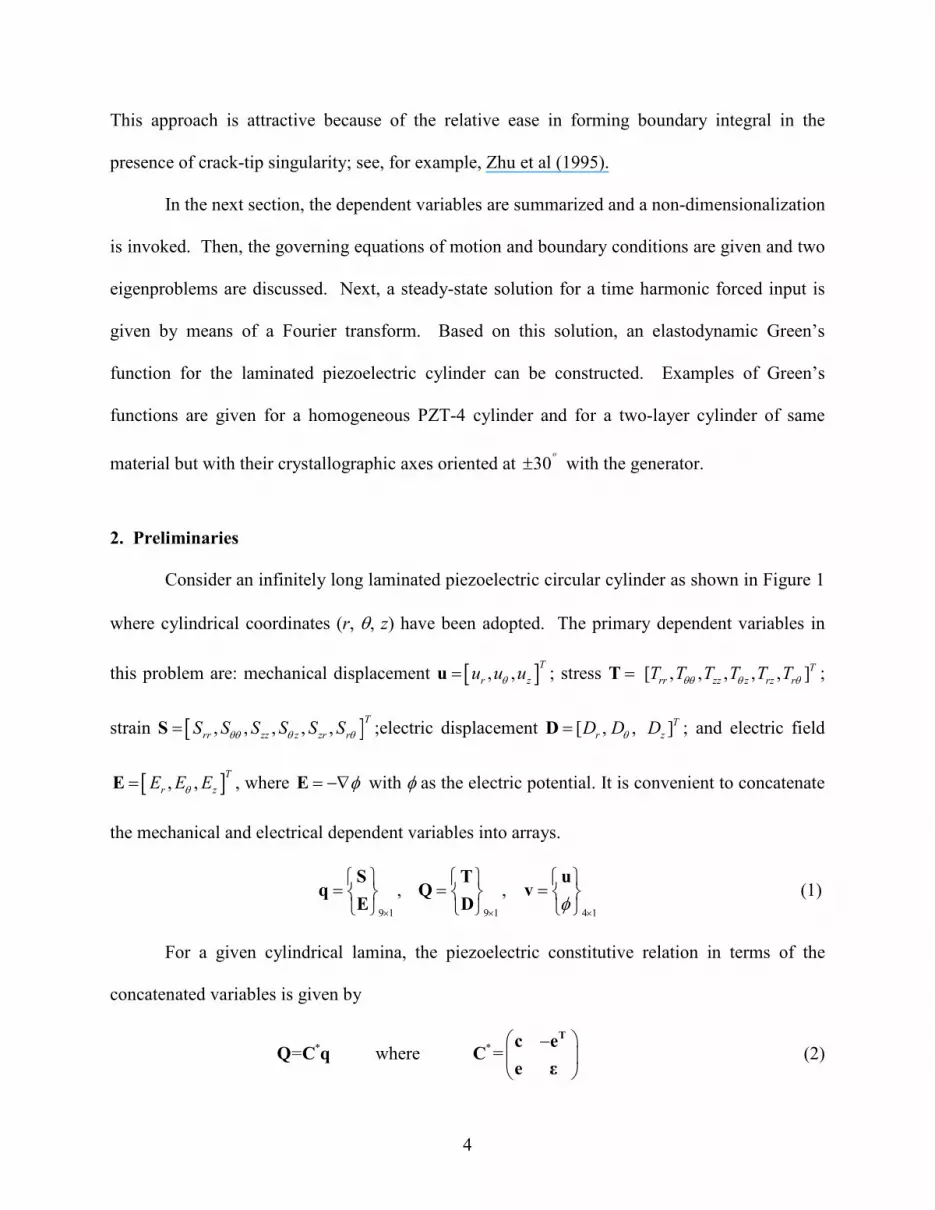
Title:Elastodynamic Green's functions for a laminated piezoelectric cylinder

Author:Bai, HTaciroglu, EDong, S B, Univeristy of California, Los AngelesShah, A H

Publication Date:11-01-2004

Publication Info:Postprints, UC Los Angeles

Permalink:http://escholarship.org/uc/item/69k6h36h

Additional Info:The original publication is available in International Journal of Solids and Structures.

Keywords:elastodynamic Green's functions, laminated piezoelectric circular cylinder, modal superposition

Abstract:Elastodynamic Green's functions for a piezoelectric structure represent the electro-mechanicalresponse due to a steady-state point source as either a unit force or a unit charge. Herein,Green's functions for a laminated circular piezoelectric cylinder are constructed by means of thesuperposition of modal data from the spectral decomposition of the operator of the equationsgoverning its dynamic behavior. These governing equations are based on a semi-analytical finiteelement formulation where the discretization occurs through the cylinder's thickness. Examples ofa homogeneous PZT-4 cylinder and a two-layer cylinder composed of a PZT-4 material at crystalorientations of +/-30degrees with the longitudinal axis are presented. Numerical implementationdetails for these two circular cylinders show the convergence and accuracy of these Green'sfunctions. (C) 2004 Elsevier Ltd. All rights reserved.

1

Elastodynamic Green’s Functions for a Laminated Piezoelectric Cylinder

H. Bai 1 , E. Taciroglu 2 , S.B. Dong 2 , and A.H. Shah 3

Abstract

Elastodynamic Green’s functions for a piezoelectric structure represent the electro-

mechanical response due to a steady state point source as either a unit force or a unit charge.

Herein, Green’s functions for a laminated circular piezoelectric cylinder are constructed by

means of the superposition of modal data from the spectral decomposition of the operator of the

equations governing its dynamic behavior. These governing equations are based on a semi-

analytical finite element formulation where the discretization occurs through the cylinder’s

thickness. Examples of a homogeneous PZT-4 cylinder and a two layer cylinder composed of a

PZT-4 material at crystal orientations of 30o± with the longitudinal axis are presented.

Numerical implementation details for these two circular cylinders show the convergence and

accuracy of these Green’s functions.

1- Lakehead University, Thunder Bay, Ontario, Canada; 2 – University of California, Los

Angeles, California, USA; 3 – The University of Manitoba, Winnipeg, Manitoba, Canada.

Corresponding author: S.B. Dong, Dept. of Civil and Envrn. Engr., University of California, Los

Angeles, 2066 Engineering I, Los Angeles, CA., 90095-1593. email dong@seas.ucla.edu

2

1. Introduction

Free vibration analysis of a structure, or alternatively the spectral decomposition of the

operator of its governing equation, yields modal data, which can be used to characterize the

structural response due to a myriad of forced inputs. Herein, we are concerned with the

construction of Green’s functions for a laminated circular cylinder based on modal data

established by the procedure of Siao et al (1994). The cylinder under consideration may be

composed of any number of uniform thickness piezoelectric layers, where each layer may have

its own material properties. The availability of Green’s functions will enable methods to be

formulated for examining the wave scattering phenomena in such cylinders in the presence of

flaws such as cracks and delaminations. It is hoped that useful ideas for structural health

monitoring will emerge from this path of investigation.

The free axisymmetric and flexural vibrations of a circular piezoelectric cylinder whose

material belongs to crystal class 6mm were first studied by Paul (1962,1966). Numerical

exploration of his frequency equations in the long wave length regime was first attempted by

Paul and Raju (1981,1982) by means of asymptotic analysis. Subsequently, Paul and

Venkatesan (1987) provided numerical data for a wide range of wave lengths under various

combinations of opened and shorted circuit conditions on the two lateral surfaces of a hollow

cylinder. Ding et al (1997) and Chen et al (2004) presented analytic solutions for the free

vibration of piezoelectric cylinders filled with a compressible fluid, wherein results for a cylinder

without fluid were also given. Buchanan and Peddieson (1989, 1991) computed the natural

frequencies of propagating waves for infinitely long piezoelectric cylinders using a one-

dimensional finite element model in the radial direction. Siao et al (1994), employing the same

radial discretization procedure and a semi-analytical finite element formulation, determined

3

spectral data for both propagating waves and edge vibrations in such cylinders. More recently,

Hussein and Heyliger (1998) presented a free vibration analysis of laminated piezoelectric

cylindrical shells using a semi-analytical discrete-layer model. While the bulk of the literature is

concerned with free vibration analyses, some studies on forced response have appeared; see, for

example, Ding et al (2003), who considered the transient axisymmetric plane strain response of a

hollow piezoelectric cylinder. For additional references on topics related to piezoelectric

structures, see Dökmeci (1980, 1989) whose surveys elaborate on a wide range of subjects,

including many on finite element calculations.

Siao et al (1994) presented a method for determining the eigendata for a circular

laminated piezoelectric cylinder. Such data consist of a finite basis of propagating waves and

edge vibrations, as contrasted with an infinity of these eigenmodes had an analytical solution

procedure been used. Nevertheless, such numerical eigendata can be made as accurate as

necessary by appropriate discretization of the thickness profile. Since one-dimensional elements

are used, the computational cost associated with a very fine model is modest vis-a-vis models

based on multi-dimensional interpolations. Herein, we utilize this method to establish the

eigendata for construction of an elastodynamic steady-state Green function for such a cylinder.

This construction is based on a modal representation of a singular source term. Examples of

such Green’s functions for two-dimensional laminated anisotropic plates and laminated

anisotropic circular cylinders were given by Zhu et al (1995) and Zhuang et al (1999),

respectively. Green’s function is essential to quantitative non-destructive evaluations of crack

sizes and locations, delaminations, and other flaws in a structure. They are used to describe the

loading conditions on the flaws and they comprise the kernels in boundary element analyses.

4

This approach is attractive because of the relative ease in forming boundary integral in the

presence of crack-tip singularity; see, for example, Zhu et al (1995).

In the next section, the dependent variables are summarized and a non-dimensionalization

is invoked. Then, the governing equations of motion and boundary conditions are given and two

eigenproblems are discussed. Next, a steady-state solution for a time harmonic forced input is

given by means of a Fourier transform. Based on this solution, an elastodynamic Green’s

function for the laminated piezoelectric cylinder can be constructed. Examples of Green’s

functions are given for a homogeneous PZT-4 cylinder and for a two-layer cylinder of same

material but with their crystallographic axes oriented at 30o± with the generator.

2. Preliminaries

Consider an infinitely long laminated piezoelectric circular cylinder as shown in Figure 1

where cylindrical coordinates (r, θ, z) have been adopted. The primary dependent variables in

this problem are: mechanical displacement [ ], , Tr zu u uθ=u ; stress =T [ , , , , , ]T

rr zz z rz rT T T T T Tθθ θ θ ;

strain [ ], , , , , Trr zz z zr rS S S S S Sθθ θ θ=S ;electric displacement [ , ,rD Dθ=D ]T

zD ; and electric field

[ ], , Tr zE E Eθ=E , where φ= −∇E with φ as the electric potential. It is convenient to concatenate

the mechanical and electrical dependent variables into arrays.

9 1 9 1 4 1

, , φ× × ×

= = = S T uq Q vE D (1)

For a given cylindrical lamina, the piezoelectric constitutive relation in terms of the

concatenated variables is given by

*=Q C q where * = − Tc eC e ε (2)

5

with c, e and εεεε as the matrices of the elastic anisotropic moduli (6×6), piezoelectric constants

(3×6) and dielectric constants (3×3), respectively. Also, there are nine generalized deformational

relations, =q Lv , where operator L contains the linear cylindrical coordinates differential

operators relating the strain and electric field to the mechanical displacement and potential

Dimensionless variables are used herein to preclude numerical anomalies due to large

differences in the units between the various material properties. In setting forth this non-

dimensionalization, regard all quantities on the right-hand and left-hand sides, respectively, of

each defining equation to be the dimensional and their corresponding dimensionless form. Four

key properties are selected as the reference values, viz., (1) total cylinder thickness h, (2) an

elastic modulus , 0c , (3) a piezoelectric constant 0e , and (4) mass density 0ρ where 0c , 0e and

0ρ are of a particular laminate in the cylinder’s radial profile. The geometry and mechanical

displacements, the material constants and mass densities are normalized as

, , ,ii

ur zr z uh h h= = = ( , , )i r zθ= (3)

0 0 0 0, , ,ε ρε ρε ρpq ij ip i

pq ij ip ic ec ec e= = = = , ( , 1, 2,3,.....,6)p q = ; ( , 1,2,3)i j = (4)

where 0ε is the reference dielectric constant given by 0 2 0( )ε oe c= . Introduce E0 and t0 as 0

00 ,cE e=

00

0ρt hc= (5)

With these parameters, time t and electric potential φ take the non-dimensional forms

0tt t= and 0E h

φφ = (6)

All of the other variables are rendered dimensionless by

( )0 , , 1, 2, ,6pp p p

TT S S pc= = = L ; ( )0 0, , 1,2,3k kk k

D ED E ke E= = = (7)

Lastly, the normalized charge ρe and body force density component if are given by

6

( )0 0, , , ,ρρ θe ie i

h h ff i r ze c= = = (8)

This non-dimensionalization scheme yields all dimensionless equations in the same form as their

dimensional counterparts.

3. Governing Equation and Boundary Conditions

The equations of motion in Siao et al (1994) are based on a semi-analytical finite element

formulation, where the discretization of the laminated cylinder takes the form of a series of three-

node cylindrical laminas, each capable of having its own piezoelectric properties and thickness.

In each three-node element, a quadratic interpolation field is used radially but the axial,

circumferential and time dependencies are left undetermined at the outset. Hamilton’s principle

with Tiersten’s (1969) electric enthalpy as the energy functional was used to derive the following

matrix equations of motion.

..

1 2 3 4 5 6+ , + , - , - , - , + =θ θθ θz z zzK V K V K V K V K V K V M V F (9)

where V is an ordered set of nodal variables for all of the nodes in the finite element model of the

cylinder. The stiffness and consistent mass matrices, i'sK and, M can be found in Siao et al

(1994), where 1 4, 5,K K K and 6K are symmetric, while 2K and 3K are antisymmetric. The

consistent load F is obtained by integrating the product of the radial interpolation functions and

the mechanical loads and electric charge over the radial profile of the cylinder.

T

errdrρ

= − ∫ fF N (10)

where f contains the components of the mechanical load and eρ is the charge density.

7

Homogeneous boundary conditions on the lateral surfaces and end cross-section can be

stated as follows. For a hollow cylinder with inside and outside radii, inr and outr , traction-free

surfaces require that

0rr r zrT T Tθ= = = (11)

The electrical condition may take the form of an opened circuit (surface is uncoated) where the

radial electric displacement component rD must vanish or a shorted-circuited condition (a coated

lateral surface that is grounded) where the potentialφ (or voltage) vanishes

rD 0= or 0φ = (12)

4. Free Vibration Analyses

For free vibrations, the solution form is

exp{ ( )}m mi k z m tθ ω= + −V V (13)

where ω is the circular frequency, ( , )mk m are the axial and circumferential wave numbers, and

mV is the array of nodal coordinates in the radial profile of the finite element discretization.

Substitution of solution form (13) into the homogeneous form of Eq. (9) gives

2 2 21 2 3 4 5 6( + + ) =0m m m m mim ik m mk k ω+ + + −K K K K K K V MV (14)

For circumferential periodicity, integer values must be used for circumferential mode number m.

Two eigenproblems can be deduced depending on whether 2ω or mk is chosen as the eigenvalue.

If 2ω is taken as the eigenvalue, then wave number mk assumes assigned values in Eq.

(14). This system is Hermitian, since the real and purely imaginary matrices are symmetric and

antisymmetric, respectively, and only real eigenvalues 2ω are admitted. Doubling the algebraic

eigensystem size reveals its real, symmetric positive-definiteness.

8

2 221 4 5 6 2 3

2 22 3 1 4 5 6

0-( + )0( + ) ω + + + = − −+ + +

V VMK K K K Κ KV VMΚ K K K K K

m mm m m

m mm m m

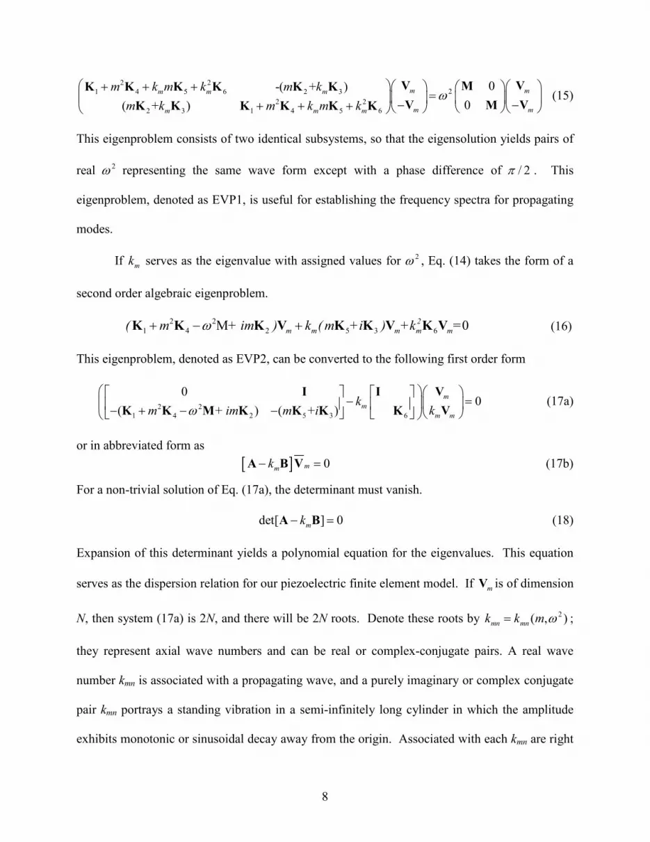
m k m k m km k m k m k (15)

This eigenproblem consists of two identical subsystems, so that the eigensolution yields pairs of

real 2ω representing the same wave form except with a phase difference of / 2π . This

eigenproblem, denoted as EVP1, is useful for establishing the frequency spectra for propagating

modes.

If mk serves as the eigenvalue with assigned values for 2ω , Eq. (14) takes the form of a

second order algebraic eigenproblem.

2 21 4 2 5 3 6 02

m m m m m( m + im ) k ( m +i ) +k =ω+ − Μ +K K K V K K V K V (16)

This eigenproblem, denoted as EVP2, can be converted to the following first order form

2 21 4 2 5 3 6

0 0( + ) ( + )m

mm m

km im m i kω − = − + − −

I I VK K M K K K K V (17a)

or in abbreviated form as

[ ] 0mmk− =A B V (17b) For a non-trivial solution of Eq. (17a), the determinant must vanish.

det[ ] 0mk− =A B (18)

Expansion of this determinant yields a polynomial equation for the eigenvalues. This equation

serves as the dispersion relation for our piezoelectric finite element model. If Vm is of dimension

N, then system (17a) is 2N, and there will be 2N roots. Denote these roots by 2( , )mn mnk k m ω= ;

they represent axial wave numbers and can be real or complex-conjugate pairs. A real wave

number kmn is associated with a propagating wave, and a purely imaginary or complex conjugate

pair kmn portrays a standing vibration in a semi-infinitely long cylinder in which the amplitude

exhibits monotonic or sinusoidal decay away from the origin. Associated with each kmn are right

9

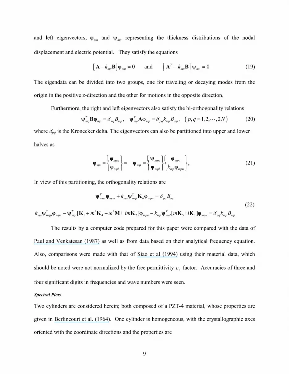
and left eigenvectors, mnφ and mnψ representing the thickness distributions of the nodal

displacement and electric potential. They satisfy the equations

[ ] 0mn mnk− =Α Β φ and 0Tmn mnk − = Α Β ψ (19)

The eigendata can be divided into two groups, one for traveling or decaying modes from the

origin in the positive z-direction and the other for motions in the opposite direction.

Furthermore, the right and left eigenvectors also satisfy the bi-orthogonality relations ( ), , , 1,2, , 2T T

mq mp pq mp mq mp pq mp mpB k B p q Nδ δ= = =ψ Βφ ψ Aφ L (20) where δpq is the Kronecker delta. The eigenvectors can also be partitioned into upper and lower

halves as

,mpu mpu mpump mp

mpl mpl mp mpuk = = = φ ψ φφ ψφ ψ φ (21)

In view of this partitioning, the orthogonality relations are

6

2 21 4 2 5 3[ + ] [ + ]

T Tmqu mpu mp mql mpu pq mp

T T Tmp mqu mpu mql mpu mp mql mpu pq mp mp

k B

k m im k m i k B

δ

ω δ

+ =

− + − − =

ψ φ ψ K φ

ψ φ ψ K K M K φ ψ K K φ(22)

The results by a computer code prepared for this paper were compared with the data of

Paul and Venkatesan (1987) as well as from data based on their analytical frequency equation.

Also, comparisons were made with that of Siao et al (1994) using their material data, which

should be noted were not normalized by the free permittivity oε factor. Accuracies of three and

four significant digits in frequencies and wave numbers were seen. Spectral Plots

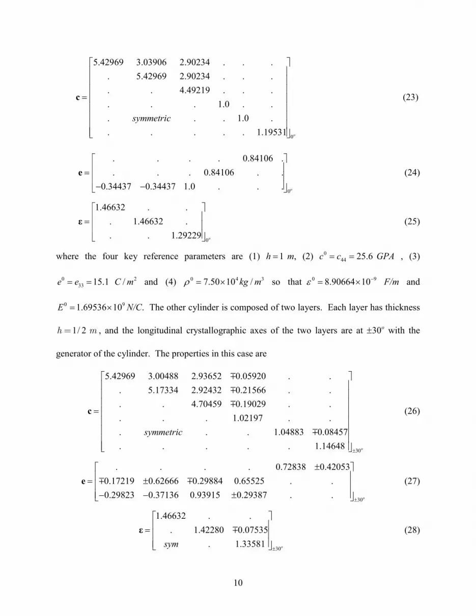
Two cylinders are considered herein; both composed of a PZT-4 material, whose properties are

given in Berlincourt et al. (1964). One cylinder is homogeneous, with the crystallographic axes

oriented with the coordinate directions and the properties are

10

0

5.42969 3.03906 2.90234 . . .. 5.42969 2.90234 . . .. . 4.49219 . . .. . . 1.0 . .. . . 1.0 .. . . . . 1.19531 o

symmetric

=

c (23)

0

. . . . 0.84106 .

. . . 0.84106 . .0.34437 0.34437 1.0 . . . o

= − − e (24)

0

1.46632 . .. 1.46632 .. . 1.29229 o

= ε (25)

where the four key reference parameters are (1) 1h = m, (2) 044 25.6c c= = GPA , (3)

033 15.1e e= = 2/C m and (4) 0 4 37.50 10 /kg mρ = × so that 0 98.90664 10ε −= × F/m and

0 91.69536 10E = × N/C. The other cylinder is composed of two layers. Each layer has thickness

1/ 2h m= , and the longitudinal crystallographic axes of the two layers are at 30o± with the

generator of the cylinder. The properties in this case are

30

5.42969 3.00488 2.93652 0.05920 . .. 5.17334 2.92432 0.21566 . .. . 4.70459 0.19029 . .. . . 1.02197 . .. . . 1.04883 0.08457. . . . . 1.14648 o

symmetric±

=

c

mmm

m

(26)

30

. . . . 0.72838 0.420530.17219 0.62666 0.29884 0.65525 . .0.29823 0.37136 0.93915 0.29387 . . o±

± = ± − − ± e m m (27)

30

1.46632 . .. 1.42280 0.07535

. 1.33581 osym ±

= ε m (28)

11

Based on these values, the normalized frequency is given by

o

ωω ω= where 0 01 / 584.24o chω ρ= = rad/sec. (29)

Using a finite element model of 30 elements for the homogeneous PZT-4 cylinder,

spectral data for circumferential mode numbers 0,1m = and shorted conditions on the inside and

outside lateral surfaces were determined. In Figure 2, three-dimensional spectral plots for the

homogeneous cylinder for circumferential mode numbers m=0 and m=1 with shorted circuit

lateral surface conditions are shown. In these plots, the real and imaginary wave numbers mk are

normalized by the thickness h, i.e., Re( mk h ), and Im( mk h ), and the normalized frequency is

shown. A comparison of the frequency spectra of the propagating modes for opened-opened and

shorted-shorted lateral surface conditions for ( 0,1m = ) is shown in Figure 3. Observe that there

are spectral curves with dips that signify the presence of waves with negative group velocities.

This information is useful to have in energy conservation calculations in the study of reflected

waves at the free end of a semi-infinitely long cylinder subjected to a monochromatic incident

wave. It is seen from Figure 3 that there is no difference in the torsional spectra for these two

cases. A three-dimensional plot of the frequency spectra for the two layer 30o± angle-ply

piezoelectric cylinder with opened-opened lateral surface conditions is shown in Figure 4. The

characteristics in this plot are noticeably different to that for the homogeneous cylinder.

5. Forced Response to a Steady-State Load

Let F in Eq. (9) be a time harmonic load of frequency ω. The θ-dependence of the load

and hence the response V can be expressed by Fourier series as

( ) ( ), , i t imm

mz t e z eω θθ ∞−

=−∞= ∑F F and ( ) ( ), , i t im

mm

z t e z eω θθ ∞−=−∞

= ∑V V (30)

12

Substitution of Eq. (30) into (9) and suppressing the common factors give a series of differential

equations in m, each of the form 2

2 26 5 3 1 4 22 [ ] [ ] 0m m

m md di m i m imdz dz ω+ + − + − + + =V VK K K K K M K V F (31)

where the coefficient matrices of the differential operators are Hermitian.

A Fourier transform is used here to remove the z-dependence, where the Fourier transform

pairs are

( ) ( ) ( ) ( )1, 2m mik z ik z

m m m m m m mk z e dz z k e dkπ∞ ∞−−∞ −∞= =∫ ∫v V V v% % (32)

The Fourier transform to Eq. (31) yields the algebraic equation.

( )2 2 26 5 3 1 4 2[ ] [ ]m m m mk k m i m imω+ + + + − + =K K K K K M K v f%% (33)

Equation (33) governs the m-th circumferential harmonic in the transformed domain. The first

step in the solution of Eq. (33) involves the homogeneous equation, which is in fact EVP2,

where the spectral decomposition of the governing operator provides the complete set of

eigendata. Thus, the solution of Eq. (33) can be represented by a modal summation of the right

eigenvectors, i.e., 2

1

Nm mn m

nunχ

== ∑v φ% (34)

where the coefficients χmn’s are evaluated by substituting Eq. (34) into Eq. (33) and using bi-

orthogonality relations (22). With some algebra, the solution vector mv% in terms of the upper

and lower half eigenvectors can be put into the form 2

1 ( )l

u

TNmn m

m mnn m mn mnk k B=

= −∑ ψ fv φ%

% (35)

13

The inverse Fourier transform of Eq. (35) recovers the axial dependence of the m-th

circumferential harmonic.

( ) 2

1

12 ( )

mTN

ik zmnl mm mnu m

n m mn mnz e dkk k Bπ

∞−∞=

= −∑∫ ψ fV φ%

(36)

In many problems, mf% , ,mn mnψ φ and Bmn will be independent of wave number km, so that

application of the Cauchy residue theorem yields the modal response in a straightforward way.

As the eigendata can be divided into two groups, mκ + and mκ − , according to traveling and

decaying motions from the origin along the positive and negative z-directions, then ( )m zV can be

written as

( ) mn mn

mn m mn m

T Tik z ik zmnl m mnl m

m mnu mnuk kmn mn

z i e i eB Bκ κ+ −∈ ∈= +∑ ∑ψ f ψ fV φ φ

% % (37)

6. Steady-State Green’s Function

For construction of Green’s function, consider a unit steady-state concentrated force or

charge at a source point in the cross-sectional plane z = 0 at θ = 0 and some radial distance r0 .

For convenience of discussion, let r0 coincide with a nodal surface. In representing this

concentrated source load in Eq. (9), F(θ, z) takes the form

( ) ( ) ( ) 0, z zθ δ θ δ=F F (38)

where δ(•) is the Dirac delta function. The vector F0 is used to define the location and type of

the unit point source, i.e., a unit force or a unit charge. Thus, F0 will contain zero entries

throughout except at nodal surface r = r0, where either a load with components (αr, αθ, αz) or a

unit charge αq = 1 is prescribed

14

Since our forced vibration solution procedure involves the expansion of δ(θ) in Fourier

series and it is well known that such a representation of it does not converge, it is necessary to

replace the point source by a uniform spatial pulse of intensity 0q over a narrow circumferential

wide 2r0θ0. For equivalence of a unit concentrated load, 0q is given by

0

00 0 0

0 0

11 2q r d or q rθθ θ θ− = =∫ (39)

For the case of a unit electric charge, the charge density eρ will have the corresponding form

0 0

12e rρ θ= (40)

Therefore, F(θ, z) in Eq. (38), for a unit force or unit charge, takes the form

( ) ( ), imm

mz e zθθ ∞

=−∞= ∑F F where ( ) ( )0

00 0

sin12m

mz zr mθ δπ θ=F F (41)

and its Fourier transform is

( ) 00

0 0

sin12m m

mk r mθ

π θ=f F% (42)

Substituting of Eq. (42) into Eq. (37) and considering motions only in the positive z-direction

yield the m-th circumferential mode of displacement Green function. Thus the steady-state unit

concentrated generalized force point source takes the form of a series of circular ring-like

sources. The displacement Green function is then represented by the summation of these

individual circumferential modal responses, i.e.,

( ) ( ) ( ) 00

0 0

sin , 02mn

mn m

Tik zmnl

m mnum m k mn

miz z e zr m Bκ

θπ θ +

∞ ∞

=−∞ =−∞ ∈= = ≥∑ ∑ ∑ ψ FV V φ (43)

15

7. Numerical Examples

The precision of Green’s function is tied to the number of terms used in the double series

representation. Each series entails its own issues, and they were discussed in Zhuang et al (1999)

for a mechanical cylinder. Their conclusions will be seen to apply here equally well from the

discussion of our numerical examples.

In the representation of a point load, in the circumferential direction by a uniform pulse

over a short arc length, Zhuang et al (1999) gave a plot showing the number of modes versus

pulse width for accuracies from 90% to 99%. This plot serves as guidance for a unit charge

since it is merely another point source. Even though a relatively large number of terms are

needed for representing a uniform pulse over a short circumferential distance, Zhuang et al

(1999) demonstrated that substantially fewer terms were required for comparable accuracy of the

stresses and displacements. The following examples, using the same two cylinders for which

spectral plots were given in Section 4, will show the same convergence rates. In both examples,

a normalized steady-state frequency of ω = 1.5 was used. Homogeneous PZT-4 Cylinder

In this example, both opened-opened and shorted-shorted circuit surface conditions were

considered. The unit load requires ring-like circumferential loads to be summed. With regards

to this circumferential summation for representation of the force and charge point sources acting

on the outer surface of the cylinder, these source terms were approximated by a uniform pulse

over a half circumferential width of 0.001 radians. The response was calculated with sum total

of circumferential mode numbers of m =10, 20, 40, 60, 80 and 100. As the accuracy is also

related to the discretized profile, different size models, i.e., 10, 20, 30, 40, 50 and 60 elements

were used. For all circumferential wave numbers, at least 30 elements were observed to be

16

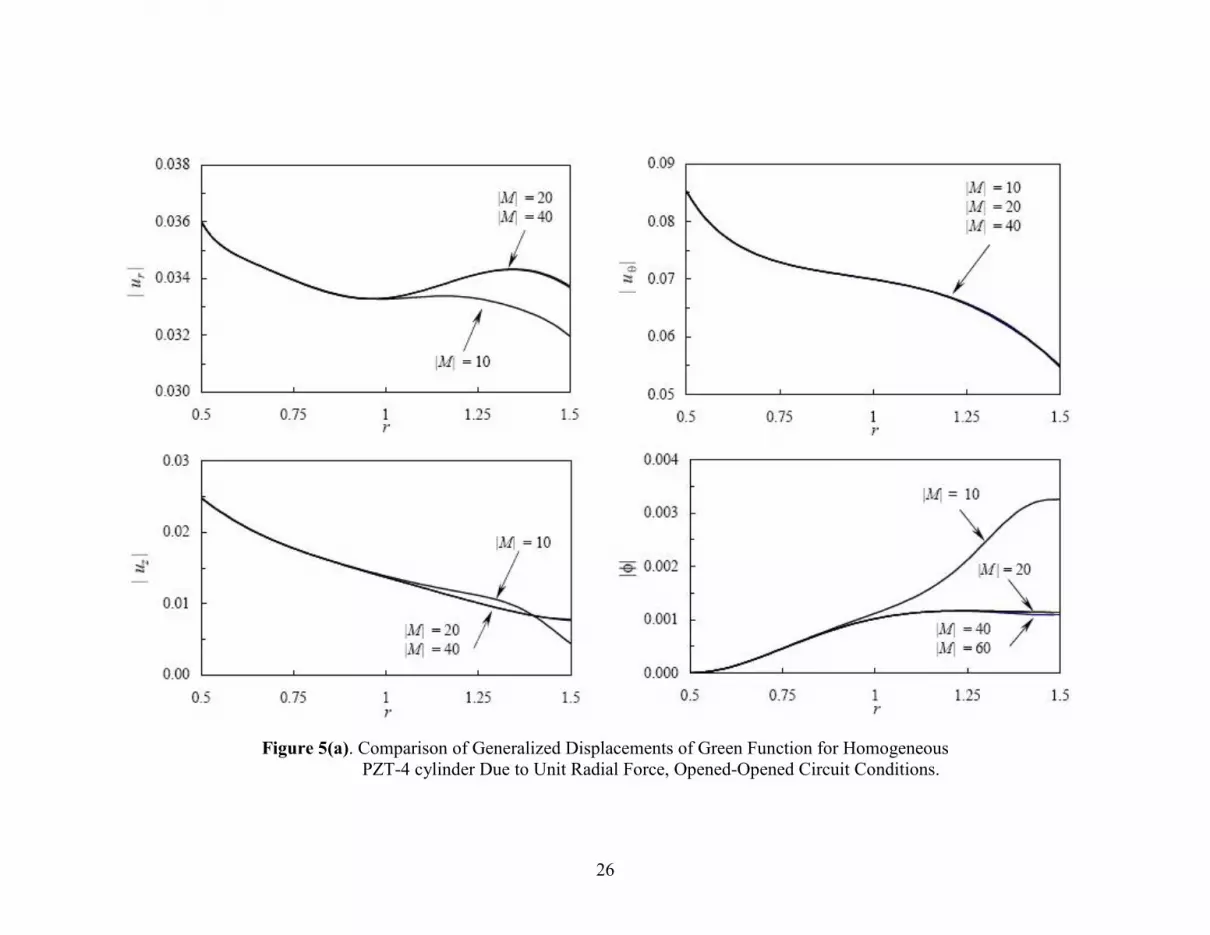
sufficient for good precision of the near-field quantities, which were examined at / 4θ π= and z

= h/4. For the specific case of a unit radial point load on the outer surface, the convergence

characteristics as a function of number of circumferential modes are shown in Figure 5(a,b).

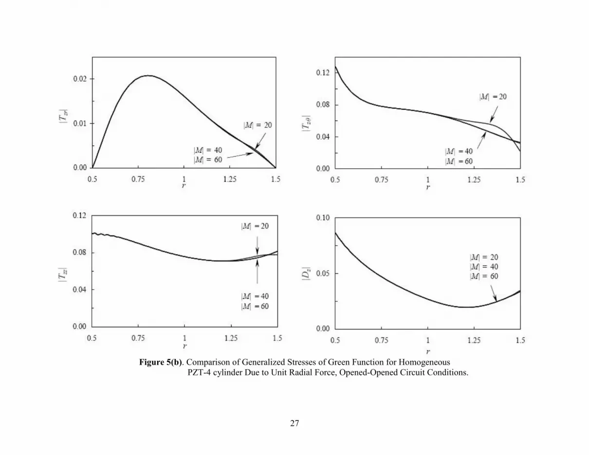
With a 30 element model, displacements and potential converged within twenty (20)

circumferential modes, and stresses and electric displacement component zD with forty (40)

modes. Sums with more than these minimum numbers of modes showed a diminishing return on

further accuracy. It is not surprising that more terms are needed for stresses than displacements

since stress calculations require differentiation of the kinematic field. In examining the balance

between the work of the ring-like source and the energy of the response field, differences of less

than 0.01% were observed for all the cases.

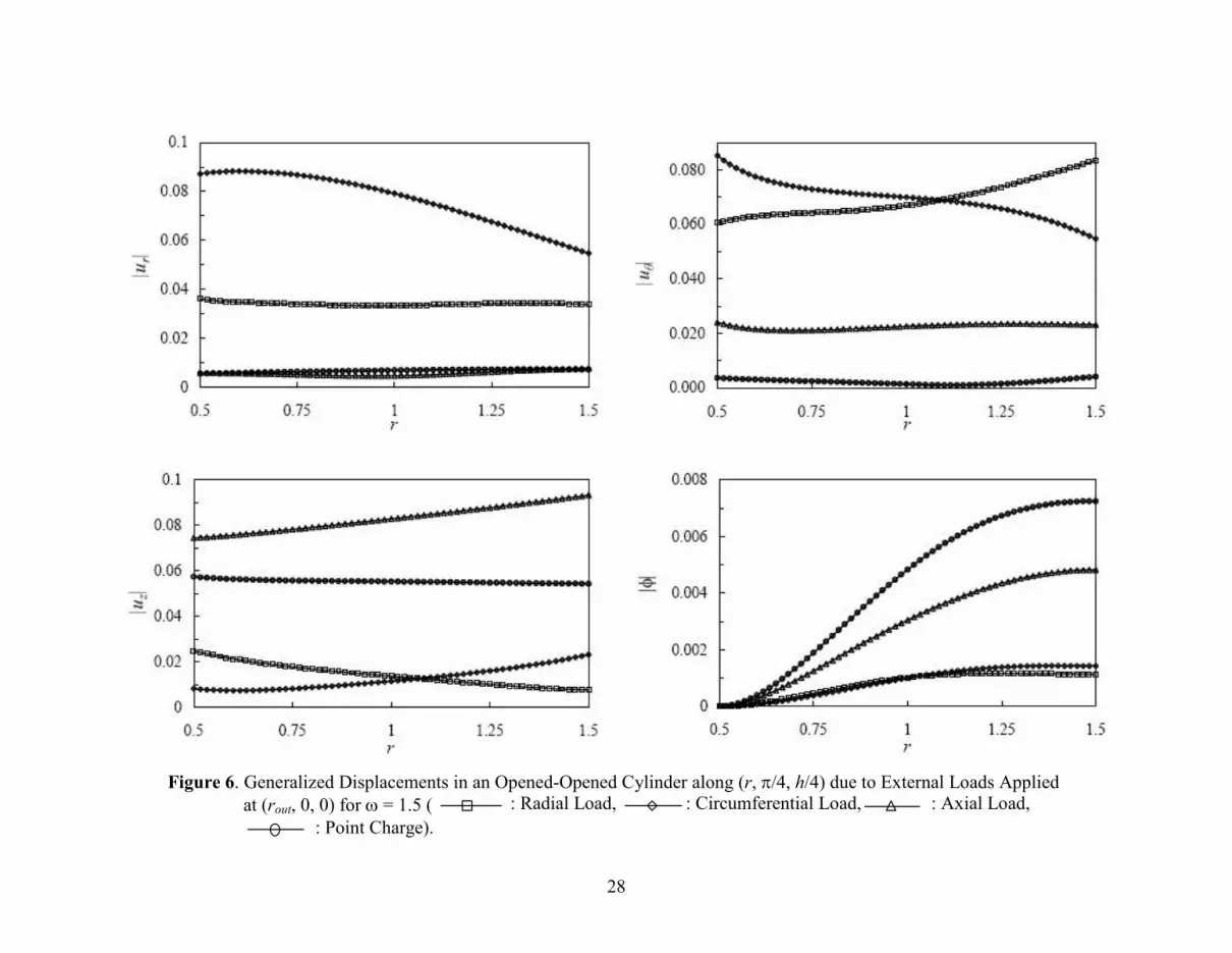
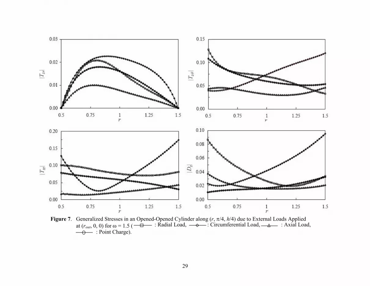
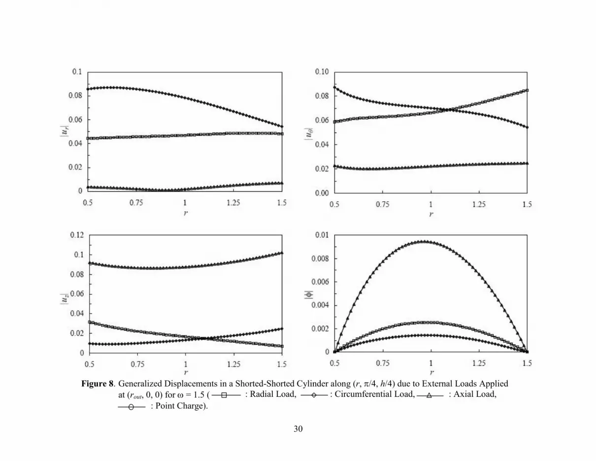
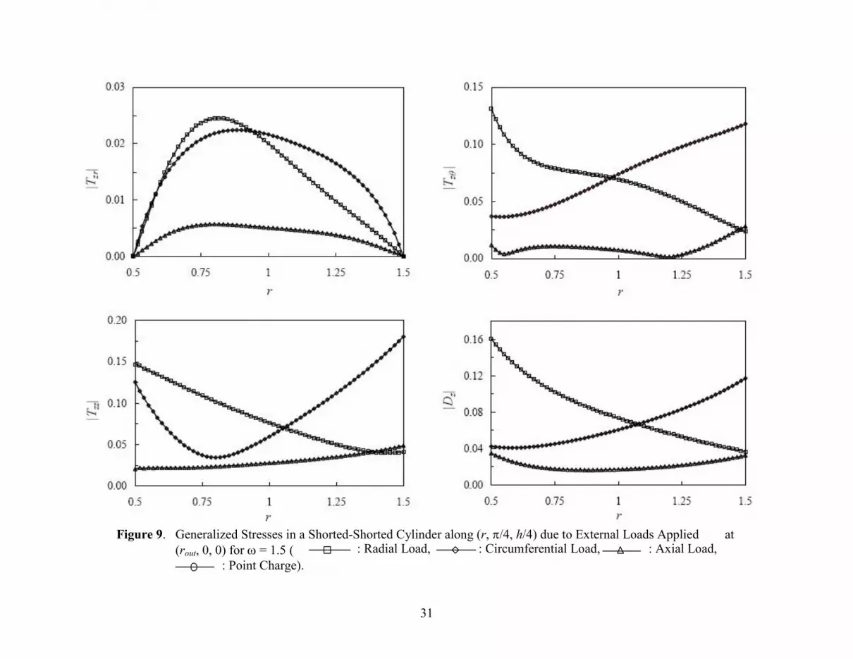
Displacement, stress, electric displacement and potential profiles at the near field location of

( ,zθ ) = (π/4, h/4) are shown in Figures 6 and 7 and Figures 8 and 9 for opened-opened and

shorted-shorted circuit conditions, respectively, and for the complete ser of point sources.

Obviously, there are no results for a surface charge in Figures 8 and 9 since the outer surface is

grounded. Also note that since the electric potential is known only to within an arbitrary

constant for the opened-opened circuit condition, the inner surface can be grounded without loss

of generality. From Figures 6 and 8, observe that the radial and circumferential displacements

dominate the response for radial and circumferential source loads, while axial displacement and

electric potential manifest greater responses for the axial point load and the electric charge. This

behavior is due to the nature of the PZT-4 material that evinces strong piezoelectric coupling

between the axial components of stress and electric field, zE . The shear stress Tzr is much

smaller than the other components as seen in Figures 7 and 9.

17

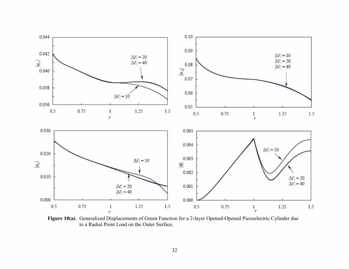
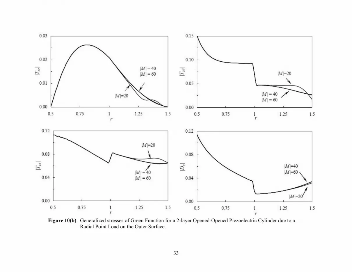
Two-Layer PZT-4 Cylinder

In this example, opened-opened lateral surface conditions were assumed. It was again found

that for a normalized steady-state frequency of ω = 1.5, 30 elements were deemed to be

sufficient for good precision of the near-field quantities. The convergence characteristics are

shown in Figures 10(a, b) for a unit radial load on the outer surface. Convergence was obtained

with essentially the same number of circumferential modes as the homogeneous PZT-4 cylinder.

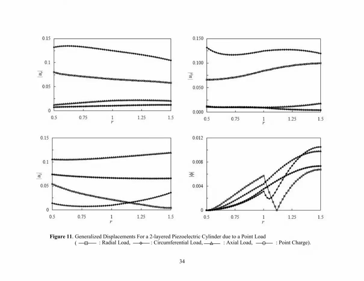
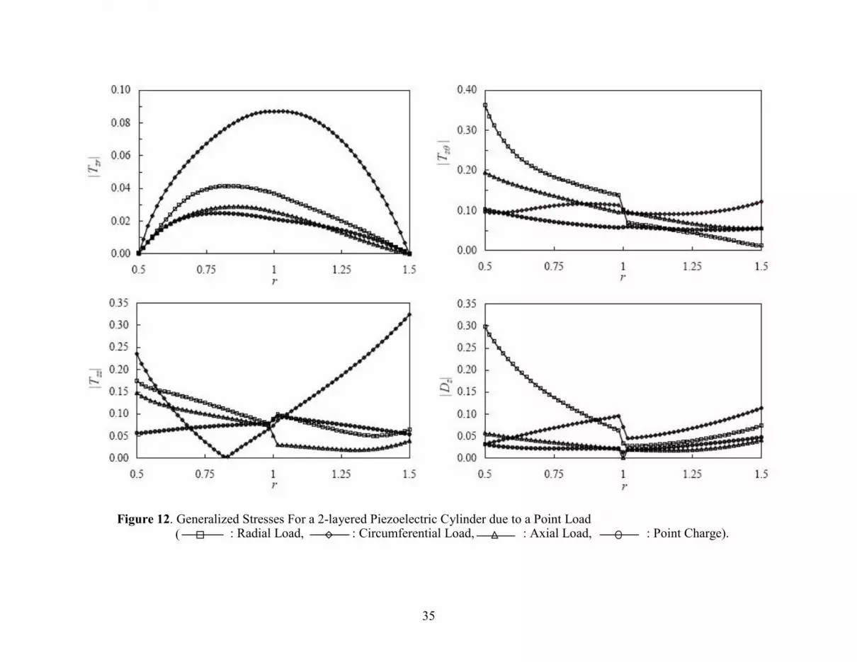
Profile plots of the displacement, stress, electric displacement and potential at the near field

location of ( ,zθ ) = (π/4, h/4) are shown in Figures 11 and 12 for the set of point loads and point

charge.

8. Conclusions

Steady-state Green functions for a laminated piezoelectric cylinder were constructed

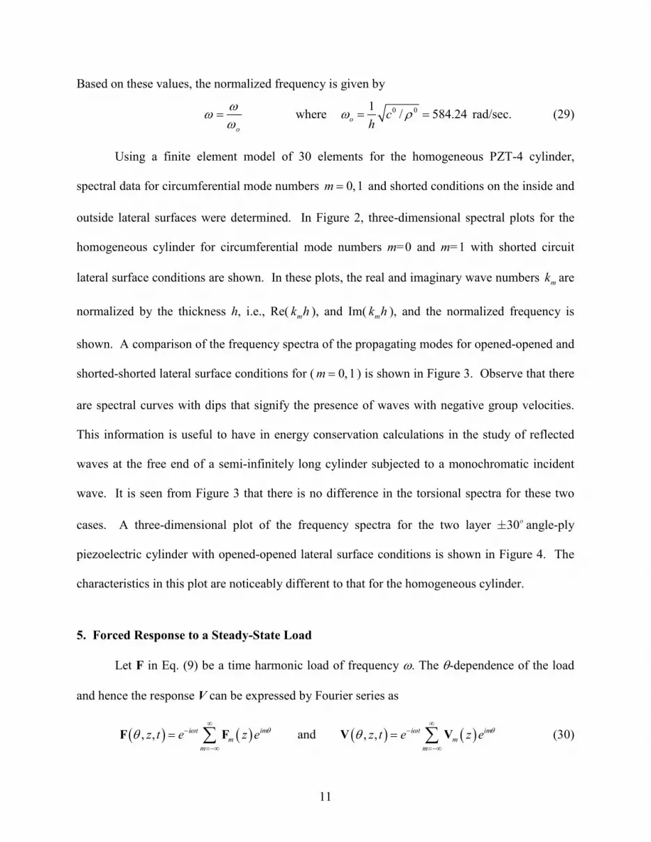
where the circumferential behavior was represented by Fourier series and the axial dependence

treated by a Fourier transform. Their implementation is based on modal data from the spectral

decomposition of the differential operator of the governing equation. Our Green’s functions are

essentially by a double summation of these data. The convergence and precision of this double

summation was discussed for the two cylinders, considering both opened-opened and shorted-

shorted electric surface conditions. The study of the convergence characteristics revealed the

necessary number of elements in the radial discretization as well as the required number of

circumferential modes for an acceptable precision of the Green’s functions depicting the four

different source terms, i.e., mechanical loads and electric charge. The required number of modes

in their representations was quite nominal and was far from being exorbitantly large. Thus,

Green’s functions in these forms should be useful in other applications.

18

References Berlincourt, D.A., Curran, D.R., and Jaffe, H., 1964, “Piezoelectric and piezomagnetic materials and their function in transducers,” Physical Acoustics, Vol. 1, Part A, 169 – 270. Buchanan, G.R. and Peddieson J. Jr., 1989, “Axisymmetric vibration of infinite piezoelectric cylinders using one-dimensional finite elements,” IEEE Transactions on Ultrasonics, Ferroelectrics and Frequency Control, 36 (4), 459 – 465. Buchanan, G.R. and Peddieson J. Jr., 1991, “Vibration of infinite piezoelectric cylinders with anisotropic properties using cylindrical finite element,” IEEE Transactions on Ultrasonics, Ferroelectrics and Frequency Control, 38 (3), 291 – 296. Chen,W.Q., Bian, Z.G., Lv, C.F. and Ding, H.J., (2004) “3D free vibration analysis of a functionally graded piezoelectric hollow cylinder filled with compressible fluid,” International Journal of Solids and Structures, 41(3-4), 947 – 964. Ding H.J., Chen, W.Q., Guo, Y.M. and Yang, Q.D., (1997), “Free vibrations of piezoelectric cylindrical shells filled with compressible fluid,” International Journal of Solids and Structures,34(16), 2025 – 2034. Ding, H.J., Wang, H.M. and Hou, P.F., 2003, “The transient response of piezoelectric hollow cylinders for axisymmetric plane strain problems,” International Journal of Solids and Structures, 40, 105 – 123. Dökmeci, M.C., 1980, “Recent advances/vibrations of piezoelectric crystals,” International journal of Engineering Science, 18, 431 - 448. Dökmeci, M.C., 1989, “Recent advances in the dynamic applications of piezoelectric crystals,” The Shock and Vibration Digest, 21, 3 - 20.

19

Hussein, M.M. and Heyliger, P.R., 1998, “Three-dimensional vibrations of layered piezoelectric cylinders,” Journal of Engineering Mechanics, 124 (11), 1294 – 1298. Paul, H.S., 1962, “Torsion vibrations of circular cylindrical shells of piezoelectric crystals,” Arch Mech. Stosowanej, 1, 123 – 133. Paul, H.S., 1966, “Vibrations of circular cylindrical shells of piezoelectric silver iodide crystals,” Journal of the Acoustical Society of America, 40 (5), 1077 - 1080. Paul, H.S. and Raju, D.P., 1981, “Asymptotic analysis of the torsional modes of wave propagation in a piezoelectric solid cylinder of (622) class,” Int. Journal of Engineering Science,19 (8), 1069-1076. Paul, H.S. and Raju, D.P., 1982, “Asymptotic analysis of the modes of wave propagation in a piezoelectric solid cylinder,” Journal of the Acoustical Society of America, 71 (3), 255 - 263. Paul, H.S. and Venkatesan, M., 1987, “Vibrations of a hollow circular cylinder of piezoelectric ceramics,” Journal of the Acoustical Society of America, 82 (3), 952 - 956. Siao, J. C-T., Dong, S.B. and Song, J., 1994, “Frequency spectra of laminated piezoelectric cylinders,” ASME Journal of Vibration and Acoustics, 116, 364 – 370. Tiersten, H.F., 1969, Linear Piezoelectric Plates, Plenum Press, New York. Zhu, J., Shah, A.H. and Datta, S.K., 1995, “Modal representation of two-dimensional elastodynamic Green’s functions,” ASCE Journal of Engineering mechanics, 121 (1), 26 – 36. Zhuang, W., Shah, A.H. and Dong, S.B., 1999, “Elastodynamic Green’s function for laminated

anisotropic circular cylinders,” ASME Journal of Applied Mechanics, 66, 665 – 673.

20

List of Figures

Figure 1 Laminated Piezoelectric Cylinder

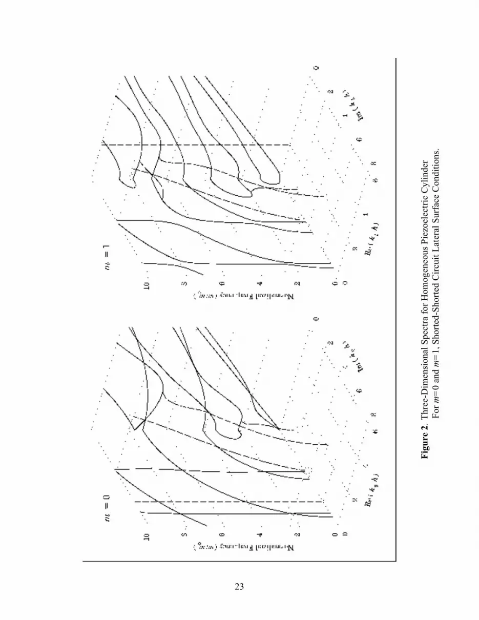
Figure 2 Three-Dimensional Spectra for Homogeneous Piezoelectric Cylinder

For m=0 and m=1, shorted-shorted circuit lateral surface conditions.

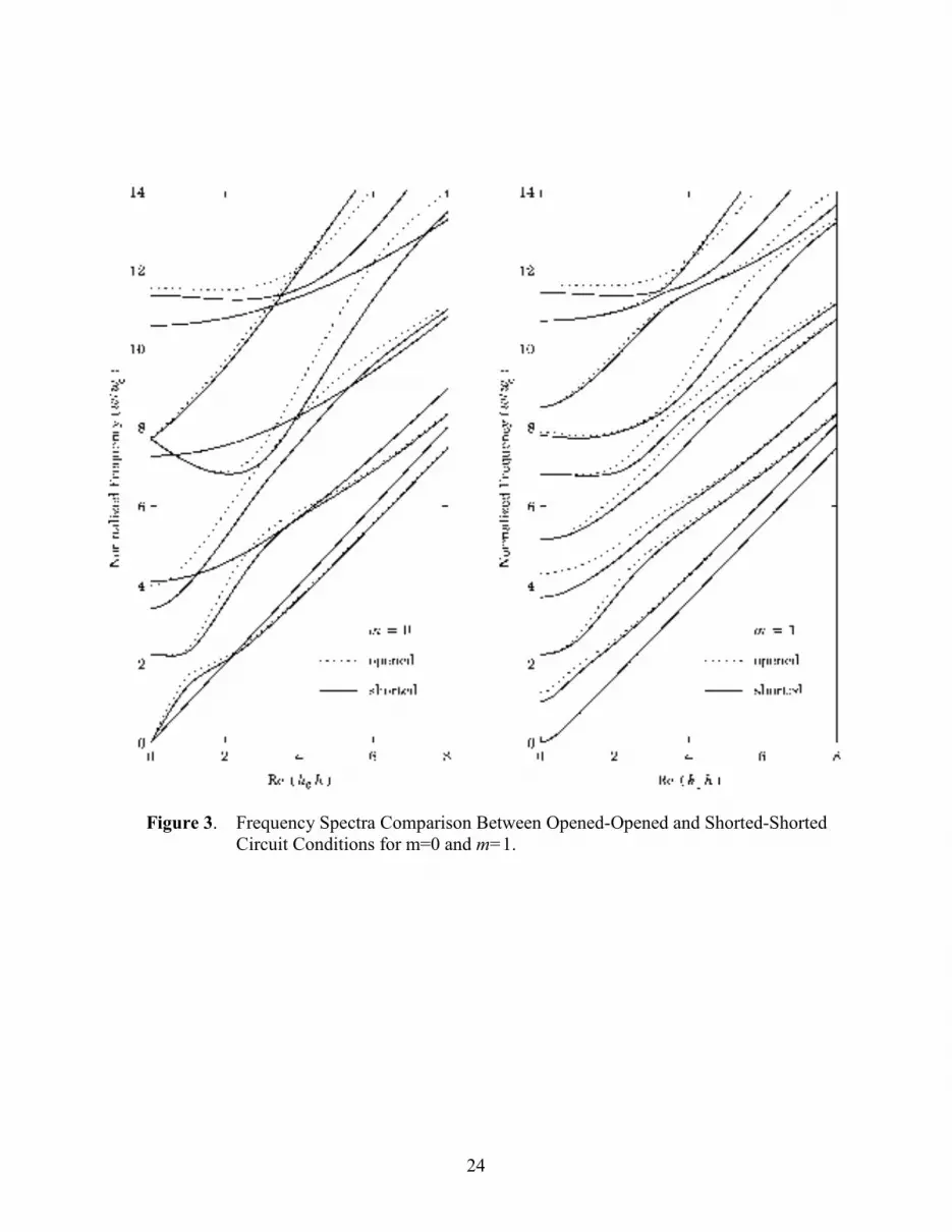
Figure 3 Frequency Spectra Comparison Between Opened-Opened and Shorted-Shorted

Circuit Conditions for m=0 and m=1

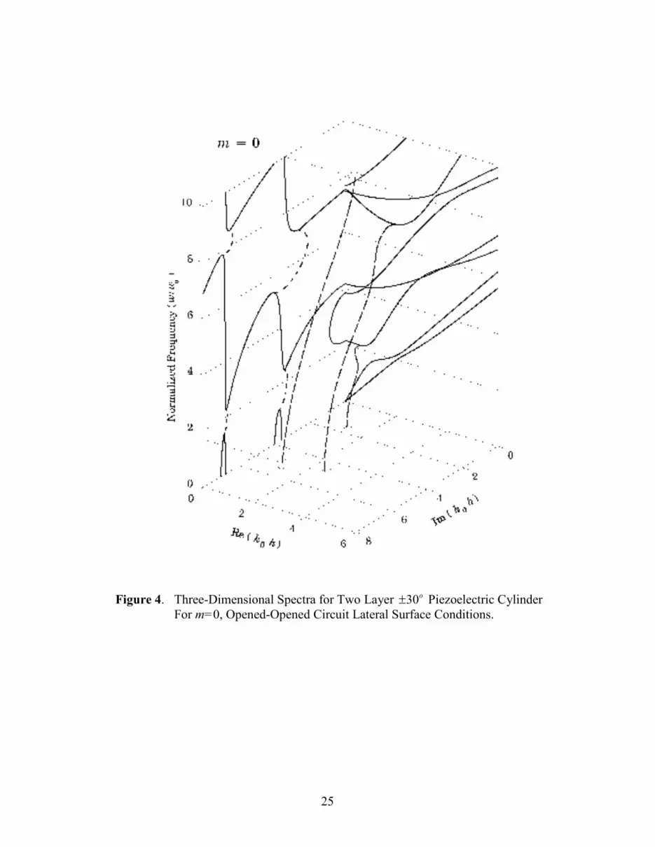
Figure 4 Three-Dimensional Spectra for Two Layer 30o± Piezoelectric Cylinder

For m=0, opened-opened circuit lateral surface conditions.

Figure 5a Comparison of Generalized Displacements of Green’s Function for Homogeneous

PZT-4 cylinder Due to Unit Radial Force, Opened-Opened Circuit Conditions

Figure 5b Comparison of Generalized Stresses of Green’s Function for Homogeneous

PZT-4 cylinder Due to Unit Radial Force, Opened-Opened Circuit Conditions

Figure 6 Generalized Displacements of Green’s Function for Homogeneous PZT-4 cylinder

Due to Unit Point Sources, Opened-Opened Circuit Conditions

Figure 7 Generalized Stresses of Green’s Function for Homogeneous PZT-4 cylinder

Due to Unit Point Sources, Opened-Opened Circuit Conditions

Figure 8 Generalized Displacements of Green’s Function for Homogeneous PZT-4 cylinder

Due to Unit Point Sources, Shorted - Shorted Circuit Conditions

Figure 9 Generalized Stresses of Green’s Function for Homogeneous PZT-4 cylinder

Due to Unit Point Sources, Shorted - Shorted Circuit Conditions

Figure 10a Comparison of Generalized Displacements of Green’s Function for Two Layer 30o±PZT-4 cylinder Due to Unit Radial Force, Opened-Opened Circuit Conditions

21

Figure 10b Comparison of Generalized Stresses of Green’s Function for Two Layer 30o±PZT-4 cylinder Due to Unit Radial Force, Opened-Opened Circuit Conditions

Figure 11 Generalized Displacements of Green’s Function for Two Layer 30o± PZT-4 cylinder

Due to Unit Point Sources, Opened-Opened Circuit Conditions

Figure 12 Generalized Stresses of Green’s Function for Two Layer 30o± PZT-4 cylinder

Due to Unit Point Sources, Opened-Opened Circuit Conditions

22

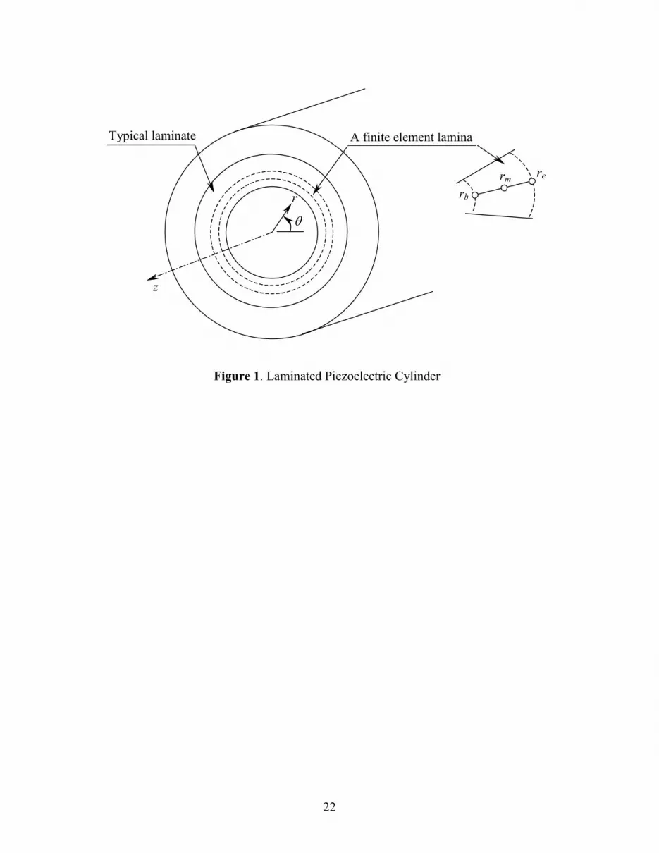
Figure 1. Laminated Piezoelectric Cylinder

θr

z

A finite element lamina Typical laminate

rm re

rb

23

Figur

e2.T

hree-D

imen

siona

lSpe

ctraf

orHo

moge

neou

sPiez

oelec

tricC

ylind

erFo

rm=0

andm

=1,S

horte

d-Sho

rtedC

ircuit

Later

alSu

rface

Cond

itions.

24

Figure 3. Frequency Spectra Comparison Between Opened-Opened and Shorted-Shorted Circuit Conditions for m=0 and m=1.

25

Figure 4. Three-Dimensional Spectra for Two Layer 30o± Piezoelectric Cylinder For m=0, Opened-Opened Circuit Lateral Surface Conditions.

26

Figure 5(a). Comparison of Generalized Displacements of Green Function for HomogeneousPZT-4 cylinder Due to Unit Radial Force, Opened-Opened Circuit Conditions.

27

Figure 5(b). Comparison of Generalized Stresses of Green Function for HomogeneousPZT-4 cylinder Due to Unit Radial Force, Opened-Opened Circuit Conditions.

28

Figure 6. Generalized Displacements in an Opened-Opened Cylinder along (r, π/4, h/4) due to External Loads Appliedat (rout, 0, 0) for ω = 1.5 ( : Radial Load, : Circumferential Load, : Axial Load,

: Point Charge).

29

Figure 7. Generalized Stresses in an Opened-Opened Cylinder along (r, π/4, h/4) due to External Loads Appliedat (rout, 0, 0) for ω = 1.5 ( : Radial Load, : Circumferential Load, : Axial Load,

: Point Charge).

30

Figure 8. Generalized Displacements in a Shorted-Shorted Cylinder along (r, π/4, h/4) due to External Loads Appliedat (rout, 0, 0) for ω = 1.5 ( : Radial Load, : Circumferential Load, : Axial Load,

: Point Charge).

31

Figure 9. Generalized Stresses in a Shorted-Shorted Cylinder along (r, π/4, h/4) due to External Loads Applied at(rout, 0, 0) for ω = 1.5 ( : Radial Load, : Circumferential Load, : Axial Load,

: Point Charge).

32

Figure 10(a). Generalized Displacements of Green Function for a 2-layer Opened-Opened Piezoelectric Cylinder dueto a Radial Point Load on the Outer Surface.

33

Figure 10(b). Generalized stresses of Green Function for a 2-layer Opened-Opened Piezoelectric Cylinder due to aRadial Point Load on the Outer Surface.

34

Figure 11. Generalized Displacements For a 2-layered Piezoelectric Cylinder due to a Point Load( : Radial Load, : Circumferential Load, : Axial Load, : Point Charge).

35

Figure 12. Generalized Stresses For a 2-layered Piezoelectric Cylinder due to a Point Load( : Radial Load, : Circumferential Load, : Axial Load, : Point Charge).