Engineering with Computers (2003) 19: 130–141 DOI 10.1007/s00366-003-0255-1 ORIGINAL ARTICLE N. V. Queipo · L. E. Zerpa · J. V. Goicochea · A. J. Verde · S. A. Pintos · A. Zambrano A model for the integrated optimization of oil production systems Received: 29 August 2001 / Accepted: 19 December Springer-Verlag London Limited 2003 Abstract Typically, the optimization of oil production systems is conducted as a non-systematic effort in the form of trial and error processes for determining the com- bination of variables that leads to an optimal behavior of the system under consideration. An optimal or near opti- mal selection of oil production system parameters could significantly decrease costs and add value. This paper presents a solution methodology for the optimization of integrated oil production systems at the design and oper- ational levels, involving the coupled execution of simul- ation models and optimization algorithms (SQP and DIRECT). The optimization refers to the maximization of performance measures such as revenue present value or cumulative oil production as objective functions, and tub- ing diameter, choke diameter, pipeline diameter, and oil flow rate as optimization variables. The reference con- figuration of the oil production system includes models for the reservoir, tubing, choke, separator, and business economics. The optimization algorithms Sequential Quadratic Programming (SQP) and DIRECT are con- sidered as state-of-the-art in non-linear programming and global optimization methods, respectively. The proposed solution methodology effectively and efficiently optimizes integrated oil production systems within the context of synthetic case studies, and holds promise to be useful in more general scenarios in the oil industry. Keywords Integrated surface and reservoir modeling and optimization · Oil production systems Nestor V. Queipo (), Luis E. Zerpa, Javier V. Goicochea, Alexander J. Verde, Salvador A. Pintos Applied Computing Institute, Faculty of Engineering, University of Zulia, Venezuela Alexander Zambrano Production Process Optimization, Av. Ernesto Blohm. Edif. PDVSA Exploracio ´n y Produccio ´n, Chuao. P.O. Box 829. Caracas 1010-A, Venezuela. Nomenclature B: Formation volume factor C D : Discharge coefficient D: Non-Darcy skin D CH :Choke diameter G: Mass flux gc : Gravitational constant h : Height of reservoir K : Absolute permeability k : Specific heat ratio, Cp/Cv k RO : Relative permeability of oil M : Molecular weight n : Politropic exponent for gas P : Absolute pressure P R : Average reservoir pressure P r : Reduced pressure q: Production rate, flow rate R : Universal gas constant r e : Radius of drainage R S : Gas-Oil ratio r w : Radius of wellbore s: Skin factor S: Saturation T : Absolute temperature T r : Reduced temperature v : Mole specific volume V: Reservoir volume V G : Specific gas volume V L : Specific liquid volume x : Free gas quality X : Mole fraction liquid phase Y : Mole fraction gas phase, pressure ratio Greek letters : Viscosity : Density : Porosity : acentric factor
Transcript
Engineering with Computers (2003) 19: 130–141DOI 10.1007/s00366-003-0255-1
ORI GI NAL AR TIC LE
N. V. Queipo · L. E. Zerpa · J. V. Goicochea ·A. J. Verde · S. A. Pintos · A. Zambrano
A model for the integrated optimization of oil production systems
Received: 29 August 2001 / Accepted: 19 December
Springer-Verlag London Limited 2003
Abstract Typically, the optimization of oil productionsystems is conducted as a non-systematic effort in theform of trial and error processes for determining the com-bination of variables that leads to an optimal behavior ofthe system under consideration. An optimal or near opti-mal selection of oil production system parameters couldsignificantly decrease costs and add value. This paperpresents a solution methodology for the optimization ofintegrated oil production systems at the design and oper-ational levels, involving the coupled execution of simul-ation models and optimization algorithms (SQP andDIRECT). The optimization refers to the maximization ofperformance measures such as revenue present value orcumulative oil production as objective functions, and tub-ing diameter, choke diameter, pipeline diameter, and oilflow rate as optimization variables. The reference con-figuration of the oil production system includes modelsfor the reservoir, tubing, choke, separator, and businesseconomics. The optimization algorithms SequentialQuadratic Programming (SQP) and DIRECT are con-sidered as state-of-the-art in non-linear programming andglobal optimization methods, respectively. The proposedsolution methodology effectively and efficiently optimizesintegrated oil production systems within the context ofsynthetic case studies, and holds promise to be useful inmore general scenarios in the oil industry.
Keywords Integrated surface and reservoir modelingand optimization · Oil production systems
Nestor V. Queipo (�), Luis E. Zerpa, Javier V. Goicochea,Alexander J. Verde, Salvador A. PintosApplied Computing Institute, Faculty of Engineering, Universityof Zulia, Venezuela
Alexander ZambranoProduction Process Optimization, Av. Ernesto Blohm. Edif.PDVSA Exploracion y Produccion, Chuao. P.O. Box 829.Caracas 1010-A, Venezuela.
Nomenclature
B: Formation volume factorCD : Discharge coefficientD: Non-Darcy skinDCH :Choke diameterG: Mass fluxgc : Gravitational constanth : Height of reservoirK : Absolute permeabilityk : Specific heat ratio, Cp/CvkRO: Relative permeability of oilM : Molecular weightn : Politropic exponent for gasP : Absolute pressurePR: Average reservoir pressurePr : Reduced pressureq: Production rate, flow rateR : Universal gas constantre: Radius of drainageRS: Gas-Oil ratiorw: Radius of wellbores: Skin factorS: SaturationT : Absolute temperatureTr : Reduced temperaturev : Mole specific volumeV: Reservoir volumeVG : Specific gas volumeVL: Specific liquid volumex : Free gas qualityX : Mole fraction liquid phaseY : Mole fraction gas phase, pressure ratio
There is increasing interest in the oil industry in decreas-ing the cost of and adding value to production processes,due to the decline of conventional oil reserves worldwideand the correspondingly high production costs. Optimiz-ation studies in the design and operation of productionfacilities are critical to address these issues.
Typically, the optimization of oil production systems isconducted as a non-systematic effort in the form of a trialand error process for determining a combination of vari-ables that leads to an optimal behavior of the system underconsideration. The development of a formal methodologyto achieve the latter is a fundamental step for the optimalor near optimal selection of production system parameters.However, there have been limited efforts in this direction.
Rosenwald and Green [1] presented an optimizationprocedure for determining the optimum locations of wellsin a reservoir, and to determine the proper sequencing offlow rates from those wells that minimized the differencebetween the production-demand curve and the flow curveactually attained. The method uses a branch-and-boundmixed-integer program in conjunction with a mathemat-ical reservoir model.
Huppler [2] developed a procedure for finding the mostprofitable gas field production policy to meet a gas salescontract, applying nonlinear programming to the overallproblem of production rate scheduling. Also, Hupplerused dynamic programming to find the best investmentschedule in each reservoir.
See and Horne [3] conducted an optimization study offield operations under a given set of technical and econ-omic constraints. The proposed methodology consisted ofa modeling phase that provides an approximately andlocally linear model of the reservoir, and an optimizationphase that uses a linear programming algorithm to optim-ize the production schedule of a reservoir for which theproducer or injector well locations have already beenfixed.
Lang and Horne [4] developed a procedure for the max-imization of oil production, using as the decision variablesthe injection rates and downhole flowing pressure. Theprocedure involves two steps: (1) the development of asurrogate model of the reservoir performance; and (2)optimization using linear and dynamic programmingalgorithms.
Carrol [5] conducted an optimization study of an oilproduction system (drainage area, well, choke, surfacefacilities), where the principal objective was to demon-strate the effectiveness of non-linear multivariate optimiz-ation techniques (modified version of the Newton methodand a direct search method called Polytope), on the maxi-mization of the economic benefits of a well, consideringas decision variables, separator pressure and tubing diam-eter.
Fujii and Horne [6] conducted an optimization study ofwell networks, where multiple production parameterswere optimized simultaneously in terms of a profit-basedobjective function, such as total oil production, net incomefrom the oil production, or oil production present value.The techniques applied in this work were Newton-typemethods, the polytope method, and a version of a geneticalgorithm. The optimization technique can be used in thedesign stage of newly developed fields or in the planningof workovers in existing fields.
Welte and Jager [7] presented IPSE (the Integrated Pro-duction Simulation Environment), a computer softwaredevelopment that creates a production system modelingenvironment where the user can quickly create a modelof a complete production system for analysis and optimiz-ation purposes.
Handley-Schachler et al. [8] introduced a simulationand optimization method for hydrocarbon production net-works based on Sequential Linear Programming (SLP). Ithas been successfully applied to a wide variety of oper-ational problems, including de-bottlenecking, optimizationof compressor strategies and determining the optimal lift-gas allocation to networks of gas lifted wells.
This paper presents a solution methodology for the opti-mization of integrated oil production systems at the designand operational levels, involving the coupled execution ofsimulation models and optimization algorithms (SQP andDIRECT). The optimization refers to the maximization ofperformance measures such as revenue present value orcumulative oil production as objective functions, and tub-ing diameter, choke diameter, pipeline diameter, and oilflow rate as optimization variables. The reference con-figuration of the oil production system includes modelsfor the reservoir, tubing, choke, separator, and businesseconomics. The optimization algorithms Sequential Quad-ratic Programming (SQP) [9] and DIRECT [10] are con-sidered to be the state-of-the-art in non-linear program-ming and global optimization methods, respectively.
Problem definition
The problem is one of optimizing an integrated oil pro-duction system, where two levels of optimization exist:design and operation. With reference to Fig. 1, it can bewritten
find x � X � Rp
such thatf(x) is maximized
132
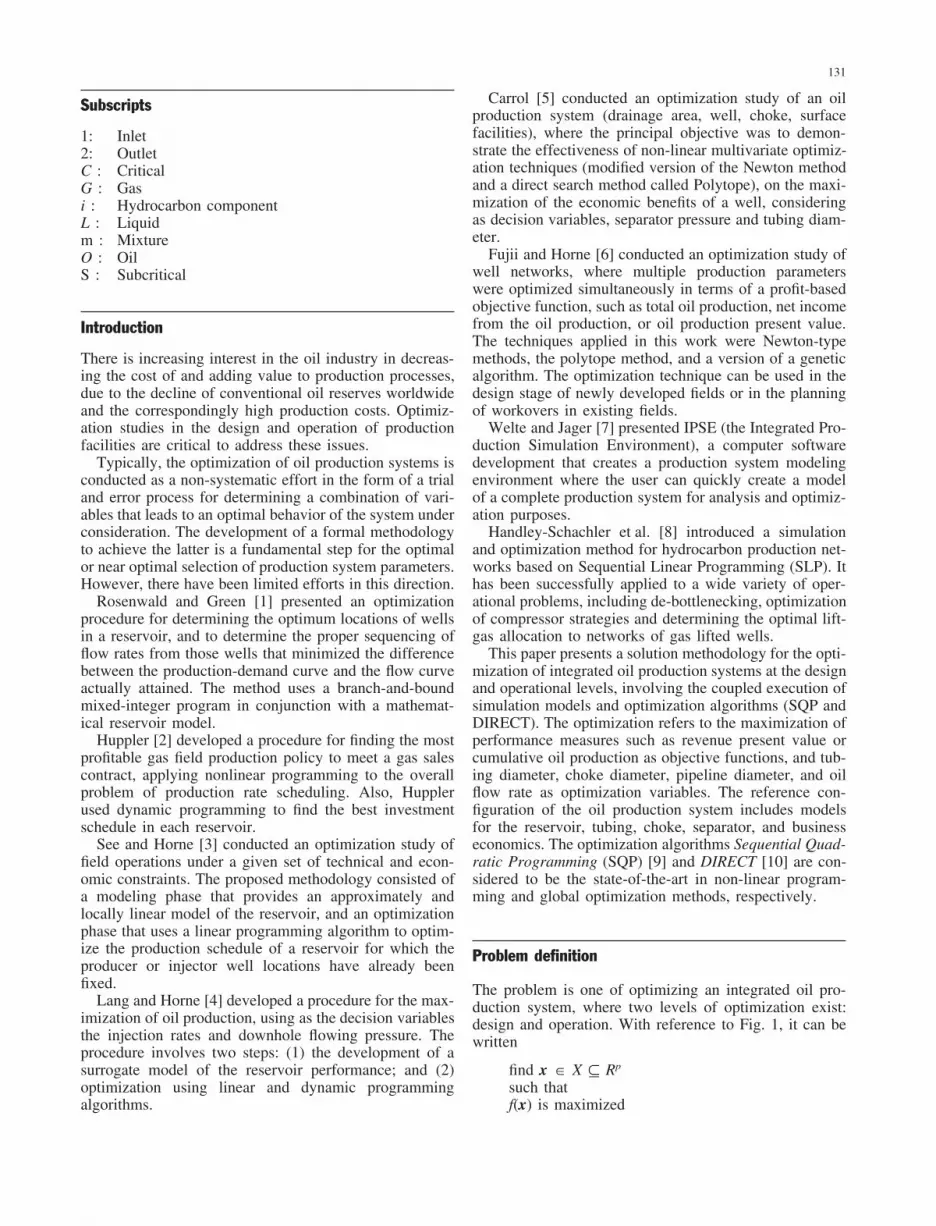
Fig. 1 Oil production system andreference configuration
where f is a mathematical function (objective function)of x, the design and/or operation variables vector (tubingdiameter, choke diameter, pipeline diameter, separatorpressure, and oil production rate), and X is the constraintsset. Hence, the problem of interest is one of finding thevector of decision variables that maximize a given per-formance measure of an oil production system, subject toa set of constraints.
Solution methodology
The proposed solution procedure involves the followingsteps:
1. Development of a simulation model of an integratedoil production system.
2. Model calibration.3. Optimization of the production process.
The simulation model is a mathematical representationof an integrated oil production system – drainage area,well, wellhead assembly, and surface facilities. Specifi-cally, the model involves several submodels, such as res-ervoir, multiphase flow in pipes, choke, separator, andbusiness economics (see Fig. 1). The model allows us toevaluate different strategies of reservoir exploitation interms of cumulative oil production and revenue present
value for a given production horizon. A brief explanationof each of the sub-models is given below:
The Reservoir Model is a mathematical representationof the dynamic behavior of fluids in the reservoir (porousmedium) in terms of pressure and saturation changes. Themodel consists of a zero-dimensional black oil simulator,based on the mass conservation equation for differentphases. The mass conservation equation for each phaserelates, for a given time interval, the cumulative mass ratein a volume, with the difference between the inflow andoutflow mass rates.
Additionally, the model calculates the flowing bot-tomhole pressure (Pwf) for different oil production rates,using the expression
�PR
Pwf� kRO
�OBO� dP = qO
[ln(re/rw) � 0.75 + s + DqO]2�Kh
(1)
The reservoir behavior is simulated by the following sol-ution procedure:
A. Establish initial reservoir pressure, initial phase satu-rations, oil production rate, and time step length.
B. Calculate the reservoir initial gas and oil mass:
Oil mass ��SO�OS
BO� V (2)
133
Gas mass ��SG�GS
BG
+�SORS�G
S
BO� V (3)
C. Determine the total oil production for the time step(�t):
�NP = qO * �t
D. Estimate the reservoir pressure at the end of thetime step.
E. Calculate the hydrocarbon properties (BO, BG, RS, �O,�G) for the gas and liquid phases at the new reser-voir pressure.
F. Calculate the oil saturation (at time level k):
V ���SO�OS
BO�
k�1
� ��SO�OS
BO�
k� = �NP (4)
G. Calculate the gas saturation:
SG = 1.0 � (SO + SW) (5)
H. Calculate the oil and gas relative permeabilities as afunction of gas saturation:
kRO = f(SG)
kRG = f(SG)
I. Update the value for oil and gas mass in the reservoirusing the saturations calculated in steps F and G.
J. Determine the total gas production for the time stepfrom the total oil production, and the average betweenthe phase mobility ratio and solution gas-oil ratio attimes k � 1 and k:
�GP = �NP *12 ��G
S �kRG�OBO
kRO�GBG
+ RS�k�1
+ �GS (6)
�kRG�OBO
kRO�GBG
+ RS�k�
K. Calculate gas material balance error, and return to stepD, until the error is less than a specified tolerance:
Error = �(MasadeGas)k�1k + �GP (7)
The hydrocarbon properties are determined as a func-tion of API gravity and reservoir pressure from empiricalcorrelations [11–15].
The reservoir model offers:
� Gas production rate.� Decline of the reservoir pressure with time.� Change of saturation of the fluids in the reservoir
with time.� Cumulative oil and gas production.� Inflow Performance Relationship Curve (IPR curve).
The reservoir model consider the following assumptions:
� The reservoir is homogeneous, isotropic, horizontal andof uniform thickness.
� Reservoir model is zero-dimensional.� There is no flux in the boundaries.� Cylindrical well model.
� The reservoir drive mechanism is solution gas drive.� The gas-oil ratio is constant throughout the reservoir.� Production occurs under pseudo-steady state con-
ditions.� Effects, such as, capillary pressure, gravity or coning
are neglected.
The Multiphase Flow Model is a mathematical rep-resentation of the fluid transport in the tubing and the hori-zontal pipeline. Specifically, it calculates the pressuredrops in the system due to the flow of multiphase fluidsfrom the bottomhole to the separator for different oil andgas rates and pipe inclinations (horizontal pipeline � =0°, vertical tubing � = 90°), using reported experimentalcorrelations [16]. Further, the model establishes the flow-ing bottomhole pressure needed to lift the fluids at differ-ent production rates for a given separator pressure.
The following algorithm calculates the pressure dropalong the hydrocarbon transport system from the well tothe separator:
Establish:
� Oil and gas production rates at standard conditions� Tubing diameter and length� Horizontal pipeline diameter and length� Choke diameter� Flowing bottomhole pressure
A. Calculate wellhead pressure, substracting from thebottomhole pressure the pressure drops along the tub-ing, and considering that fluid properties are a functionof pressure.
B. Calculate the pressure at the choke outlet, from theinlet pressure (wellhead pressure) and the oil and gasproduction rates.
C. Calculate the inlet separator pressure, from the calcu-lation of pressure drops along the horizontal pipelinefrom the choke outlet, considering that fluid propertieschange due to pressure drops.
The procedure for the calculation of pressure dropsin pipes is as follows:
a) Divide the pipe in n fragments,b) For the first fragment, determine the outlet pressure of
the element:b.1) Estimate the outlet pressure,b.2) Calculate the fluid properties using the average
pressure between the inlet and outlet,b.3) Update the oil and gas flow rates using the aver-
age pressure,b.4) Determine the flow pattern,b.5) Calculate the liquid fraction,b.6) Calculate the pressure gradient and obtain the
outlet pressure of the element,b.7) Repeat the steps b.1 to b.6 until the calculated
pressure in b.6 is equal to the pressure estimatedin b.1.
c) Repeat step (b) for the n � 1 remaining fragmentsof pipe.
The multiphase flow in pipes model estimates the fol-lowing along the pipeline system:
134
� Pressure along.� Flow pattern.� Oil production rate.� Gas production rate.
The Choke Model is a mathematical representation,originally developed by Sachdeva et al. [17], which mod-els the wellhead choke as a pipe restriction. This modelis capable of modeling critical and subcritical flow. Incritical flow, the flow rate through the choke reaches amaximum value with respect to the upstream conditionsand the fluids equal or exceed the speed of sound. Thisimplies that the flow is choked and the downstream pertur-bations are unable to propagate upstream; the opposite isalso true. For subcritical flow, the flow velocity is lessthan the speed of sound and the flow rate depends uponthe pressure drop through the device, and changes in theupstream pressure affect the downstream pressure.
The choke behavior is simulated by the following sol-ution procedure:
A. Calculate the critical pressure ratio (YC = P2/P1). Thisis done by iterating and converging on YC in the fol-lowing equation:
YC = �k
k � 1+
(1 � x) · VL · (1 � YC)x · VG1
kk � 1
+n2
+n · (1 � x) · VL
x · VG2
+n2
· �(1 � x) · VL
x · VG2�2�
kk�1
(8)
where
VG2 = VG1 · Y�1kC (9)
B. Determine the critical mass flux using the criticalpressure ratio:
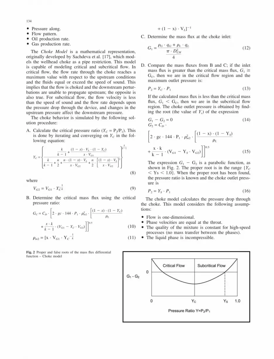
Fig. 2 Proper and false roots of the mass flux differentialfunction – Choke model
+ (1 � x) · VL]�1
C. Determine the mass flux at the choke inlet:
G1 =�G · qG + �L · qL
� · D2CH
4
(12)
D. Compare the mass fluxes from B and C; if the inletmass flux is greater than the critical mass flux, G1 GC, then we are in the critical flow region and themaximum outlet pressure is:
P2 = YC · P1 (13)
If the calculated mass flux is less than the critical massflux, G1 GC, then we are in the subcritical flowregion. The choke outlet pressure is obtained by find-ing the root (the value of Ys) of the expression
G1 � G2 = 0 (14)G2 = CD ·
�2 · gc · 144 · P1 · �2m2 · �(1 � x) · (1 � YS)
�L
+x · k
k � 1· (VG1 � YS · VG2)��0.5
(15)
The expression G1 � G2 is a parabolic function, asshown in Fig. 2. The proper root is in the range {YC
Ys 1.0}. When the proper root has been found,the pressure ratio is known and the choke outlet press-ure is
P2 = YS · P1 (16)
The choke model calculates the pressure drop throughthe choke. This model considers the following assump-tions:
� Flow is one-dimensional.� Phase velocities are equal at the throat.� The quality of the mixture is constant for high-speed
processes (no mass transfer between the phases).� The liquid phase is incompressible.
135
The Separator Model is a mathematical representationof an isothermal flash separation process or flash equilib-ria. The input of the model is the liquid and gas compo-sition at the entrance of the separator, and the output isthe liquid and gas composition, and the amount of thephases that result of the separation process, at a giventemperature and pressure of the separator [18–20].
The separation occurs in a constant pressure process,achieved by controlling the oil and gas flow that exits theseparator. The mass transfer between the phases dependson the composition of the hydrocarbon and the operationseparator conditions.
In general, the separation process consists of passingthe well stream into a separator to isolate the gas andliquid phases. The liquid phase, a result of the separationprocess, is passed to additional stages of separation thatoperate at lower pressures until it is deliver to the stocktank.
The liquid fraction recovery is improved by addingmore separators between the wellhead and the stock tank.Increasing the number of separators, the separation pro-cess is transformed from a flash liberation process to adifferential liberation process, maximizing the liquidrecovery. For a finite number of separators, there is anoptimal combination of separation pressures that maxim-ize the liquid recovery.
In this study, the separation model was implementedfor one separation stage, but it could be used to modelseveral separation stages, and to optimize the combinationof separator pressures that maximize the liquid fractionrecovery.
The procedure of performing a flash calculation is iter-ative and converges when the fugacity of each componentis the same for both phases, as follows:
A. First, determine the number of moles that enter to theseparator.Number of moles of the liquid phase:
FL =qL,1 · �L
ML
(17)
Number of moles of the gas phase:
FG =qG,1 · �G
MG
(18)
Total mole number (feed):
F = FL + FG (19)
Been X and Y the liquid and gas composition that enterthe separator, respectively.
The overall composition of the mixture that enterthe separator is represented by the followingexpression:
Zi =FL · Xi+FG · Yi
F(20)
B. Estimate the gas and liquid phase composition at theseparator pressure and temperature conditions, esti-
mating the equilibrium ratio for each component(Wilson equation), and the molar fractions for eachphase (Rachford–Rice). The equilibrium ratio (Ki) isthe ratio of gas mole fraction (Yi) to the liquid molefraction (Xi) of the component I:
Ki =Yi
Xi
(21)
B.1 The first estimate of the equilibrium ratios ismade using the Wilson equation (1962):
Ki =exp�5.37(1 + �i) �1 �
1Tri��
Pri
(22)
B.2 The Rachford–Rice equation expressed as func-tion of gas mole fraction (V) is
g(V) = �n
i=1
(Yi � Xi) = �n
i=1
Zi(Ki � 1)1 + V(Ki � 1)
= 0 (23)
The Rachford–Rice equation expressed as function ofliquid mole fraction (L) is
f(L) = �n
i=1
Zi(1 � Ki)L + (1 � L)Ki
= 0 (24)
Evaluate the Rachford–Rice equation for gas molefraction values of V = 0 and V = 1, to determine thenumber of phases present. If g(0) 0 (only liquid) orif g(1) � 0 (only gas), then for the first iteration thegas mole fraction is fixed to a value of 0.5, in sub-sequent iterations, if g(0) 0, V = 0, and if g(1) �0, then V = 1.
If g(0) � 0 and g(1) 0, there are two phases(liquid and gas). Using the Newton–Raphson methodto solve the Rachford–Rice equation, determine theliquid mole fraction (L) as follows:
Lk+1 = Lk �f(Lk)�f�L|Lk
(25)
and convergence if achieved when both
1. abs(Lk+1 � Lk) 2. f(Lk+1) where is a small tolerance.
The gas mole fraction is
V = 1 � L (26)
B.3 Determine the liquid and gas phase compo-sitions, calculating the mole fraction of the compo-nents in each phase:
Xi =Zi
[1 + V(Ki � 1)], i = 1 % n (27)
Yi =Ki · Zi
[1 + V(Ki � 1)], i = 1 % n (28)
136
C. Calculate the equation of state Soave–Redlich–Kwong(SRK) parameters from the critical pressure and tem-perature of each component (a, b, �).Equation of state SRK:
P =R · Tv � b
�a · �
v(v + b)(29)
bi = 0.08664R · Tci
Pci
(30)
ai = 0.42747R2 · T2
ci
Pci
(31)
�i = [1 + mi (1 � Tri0.5)]2 (32)
mi = 0.48 + 1.574�i � 0.176�i2 (33)
Mixing rules:
bm = �n
i=1
Xi · bi (34)
(a�)ij = (1 � kij) (a�)0.5i (a�)0.5
j (35)
where kij are the binary interaction parameters, whenall the components are hydrocarbons these parametersare zero.
(a�)m = �i
�j
Xi · Xj(a�)ij (36)
If all kij are zero:
(a�)m = ��i
Xi (a�)0.5i �2
(37)
The equation of state SRK could be expressed in acubic form as follows:
z3 � z2 + (A � B � B2) z � A · B = 0 (38)
where z is the compressibility factor, and A and B are:
A =(a�)mPR2 · T2 (39)
B =bm · PR · T
(40)
D. Solve the equation of state for the compressibility fac-tors of each phase. The major root gives the gas com-pressibility factor, and the minor positive root givesliquid compressibility factor.
E. Determine the partial fugacities of each component, ineach phase. The fugacity coefficient is given by
ln�i =bi
bm
(z � 1) � Ln(z � B) +AB � bi
bm
� 2 � (a�)i
(a�)m�1
2� Ln �1 +Bz� (41)
and the partial fugacities by
fi = Xi · �i · P (42)
F. If the partial fugacities ratio of each component is one,then the equilibrium between the two phases is achi-eved.
The procedure is assume to converge when,
�ifi,L
fi,V� 1�2
, where is a small tolerance.
If the convergence criterion is not accomplished, esti-mate new values of the equilibrium ratio as follows:
Ki =�i,L
�i,V
(43)
then proceed from step B.G. Calculate the production rates that results from the
separation process.Liquid production rate:
qL,2 =L · F · ML
�L
(44)
gas production rate:
qg,2 =V · F · MG
�G
(45)
In general, the Economic Models estimate the profits ina given time period, considering the revenues and costsinvolved [21]. These models calculate the Net PresentValue (NPV) as the present value of the revenue stream(PVrev) minus the present value of the costs (PVcost), wherethe PVrev reflects the present value of the revenue streamassociated with the produced hydrocarbon market value.The PVcost is calculated as the present value of the totalcost required to maintain the well production during agiven time period. This cost is the sum of operational costplus tax payments. The operational costs are associatedwith the operation and maintenance of the well. The costdue to tax payments is estimated based on the presentvalue of the revenue stream, and the valid tax rules. Theeconomic model developed in this study does not con-sider PVcost.
The present value of the revenue stream is determinedby the expression
PVrev = �n
i=2
[PVrevi�1+ �COPi · S · Dn] (46)
where �COPi represents the incremental oil cumulativeproduction for the ith production period, n is the numberof periods of composition over which the interest rate isapplied, S is the oil barrel price, and D is the discountfactor. This factor is calculated by the expression
D =1
1 + � ia
na� (47)
137
where ia is the interest rate and na is the number of periodsof composition per year.
The cost present value PVCost is calculated by
PVCost = PVCOper + PVtax (48)
where PVCoper and PVtax are the operational costs and taxpayments, respectively.
Usually, these costs have an annually predefined value.The increase in operational costs is determined based in anannually fixed incremental rate (IncOp), by the expression
PVCOper = COper1 + �n
i=2
(PVCOperi · IncOp · Dn)
(49)
where COper1 is the operational cost in the first year.The cost present value due to tax payments are esti-
mated by the expression
VPCImp = VPIng · Imp (50)
where Imp is the impositive rate per oil barrel produced.Finally, the net present value, NPV is determined by
NVP = PVIng � PVCost (51)
Model calibration
The model response (e.g. cumulative production, netpresent value, etc.) depends upon a series of parametersof the different submodels. These parameters differ intheir nature and the uncertainty associated with theirspecification. For example, the diameter of the well andthe average reservoir pressure are parameters of the welland the reservoir model (drainage area), respectively, thattypically exhibit different levels of uncertainty. In manycases, it is possible to reduce the uncertainty associatedwith the specification of these parameters through subsur-face and surface tests. Nevertheless, the possibility of con-ducting all the possible tests is limited by economic con-siderations. Hence, it is necessary to establish amethodology for the calibration of the model consideringproduction data, or other well known subsurface/surfacemeasures.
The proposed methodology for the simulated modelcalibration is similar to that known as ‘history matching’in reservoir simulation, and consists of formulating thecalibration problem as an optimization problem: finding aset of parameters that minimizes the difference betweenthe values calculated by the model and the correspondinghistorical ones.
Formally, the problem can be written
find x such that,
min �mj=1
wjfobs j � fcal j(x)2
subject to a set of constrictions of the form
xi min � xi � ximax i = 1, %, n
where
x: is the vector of desired model parameter values, forexample,
� Porosity (�),� Relative permeability (kro, krg) for a given phase satu-
ration,� Initial gas saturation (Sgi).
fobs and fcal: represent the historical values and the valuescalculated by the model, for example, gas production rate.w: denotes a weighting vector for specifying the level ofadjustment of the model with respect to the observed mea-sures.
The symbol . represents the norm used (e.g. eucli-dean distance) for calculation of the distance between theobserved and calculated measures.
The proposed procedure for calibrating the simulationmodel is:
� Define the set of calibration parameters. These are theparameters that are changed in the model for matchingthe model output with the corresponding observedfield values.
� Define the lower and upper bounds for the cali-bration parameters.
� Define the initial values of the calibration parameters.� Define a function, called objective function, which
measure the level of matching between the model out-put and observed field values.
Once the model of the integrated oil production systemis calibrated we might proceed with the design and oper-ations optimization process.
Optimization
The proposed solution procedure for the optimization ofthe integrated oil production system is:
� Define the design and operational parameters, their lim-its, and initial values.
� Define the objective function. In this study, the objec-tive function is the present value of the revenue stream.
� Define the model parameters that describe the pro-duction system.
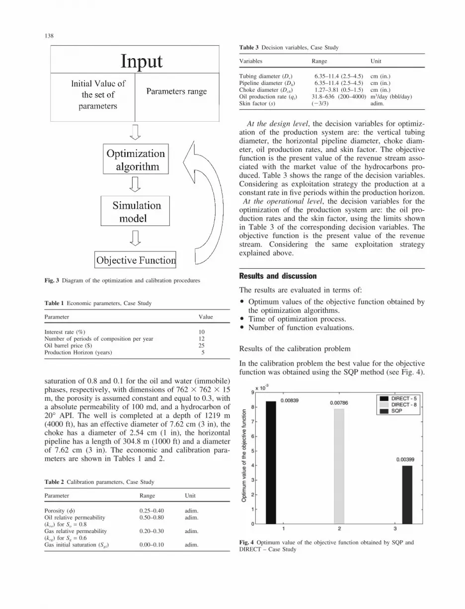
Figure 3 shows a diagram of the algorithm used forsolution of the optimization and calibration problems.
Case study
The proposed methodology is evaluated using a pro-duction system with the following characteristics: the res-ervoir (drainage area) is at a depth of 1212 m (3975 ft.),has an initial pressure of 27579 Kpa (4000 psi), a initial
138
Fig. 3 Diagram of the optimization and calibration procedures
Table 1 Economic parameters, Case Study
Parameter Value
Interest rate (%) 10Number of periods of composition per year 12Oil barrel price ($) 25Production Horizon (years) 5
saturation of 0.8 and 0.1 for the oil and water (immobile)phases, respectively, with dimensions of 762 � 762 � 15m, the porosity is assumed constant and equal to 0.3, witha absolute permeability of 100 md, and a hydrocarbon of20° API. The well is completed at a depth of 1219 m(4000 ft), has an effective diameter of 7.62 cm (3 in), thechoke has a diameter of 2.54 cm (1 in), the horizontalpipeline has a length of 304.8 m (1000 ft) and a diameterof 7.62 cm (3 in). The economic and calibration para-meters are shown in Tables 1 and 2.
Table 2 Calibration parameters, Case Study
Parameter Range Unit
Porosity (�) 0.25–0.40 adim.Oil relative permeability 0.50–0.80 adim.(kro) for So = 0.8Gas relative permeability 0.20–0.30 adim.(krg) for Sg = 0.6Gas initial saturation (Sgi) 0.00–0.10 adim.
Table 3 Decision variables, Case Study
Variables Range Unit
Tubing diameter (Dv) 6.35–11.4 (2.5–4.5) cm (in.)Pipeline diameter (Dh) 6.35–11.4 (2.5–4.5) cm (in.)Choke diameter (Dch) 1.27–3.81 (0.5–1.5) cm (in.)Oil production rate (qi) 31.8–636 (200–4000) m3/day (bbl/day)Skin factor (s) (�3/3) adim.
At the design level, the decision variables for optimiz-ation of the production system are: the vertical tubingdiameter, the horizontal pipeline diameter, choke diam-eter, oil production rates, and skin factor. The objectivefunction is the present value of the revenue stream asso-ciated with the market value of the hydrocarbons pro-duced. Table 3 shows the range of the decision variables.Considering as exploitation strategy the production at aconstant rate in five periods within the production horizon.
At the operational level, the decision variables for theoptimization of the production system are: the oil pro-duction rates and the skin factor, using the limits shownin Table 3 of the corresponding decision variables. Theobjective function is the present value of the revenuestream. Considering the same exploitation strategyexplained above.
Results and discussion
The results are evaluated in terms of:
� Optimum values of the objective function obtained bythe optimization algorithms.
� Time of optimization process.� Number of function evaluations.
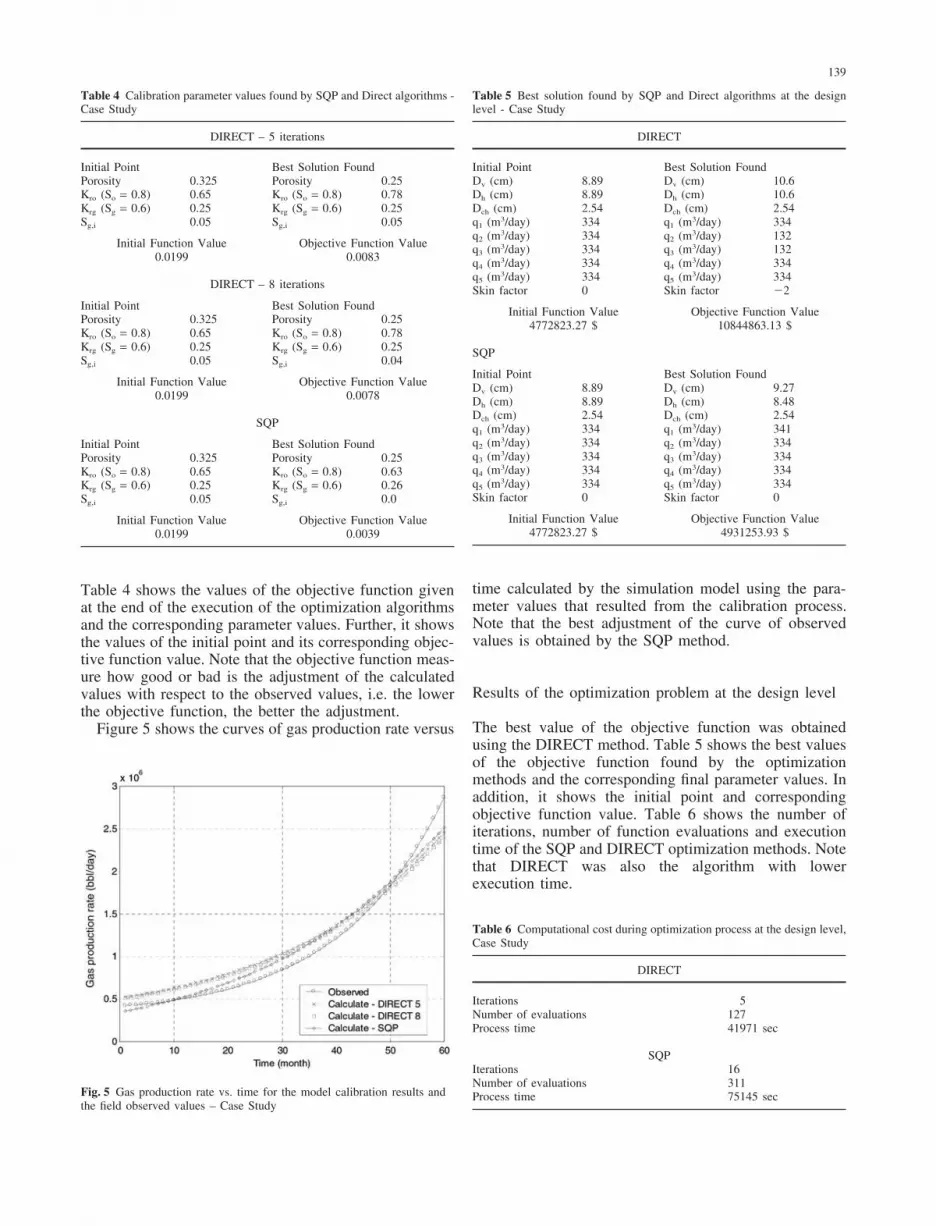
Results of the calibration problem
In the calibration problem the best value for the objectivefunction was obtained using the SQP method (see Fig. 4).
Fig. 4 Optimum value of the objective function obtained by SQP andDIRECT – Case Study
139
Table 4 Calibration parameter values found by SQP and Direct algorithms -Case Study
Initial Function Value Objective Function Value0.0199 0.0039
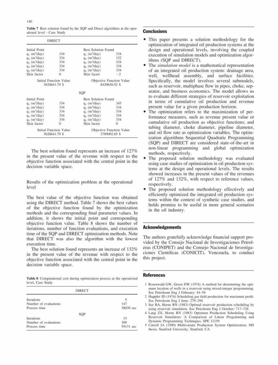
Table 4 shows the values of the objective function givenat the end of the execution of the optimization algorithmsand the corresponding parameter values. Further, it showsthe values of the initial point and its corresponding objec-tive function value. Note that the objective function meas-ure how good or bad is the adjustment of the calculatedvalues with respect to the observed values, i.e. the lowerthe objective function, the better the adjustment.
Figure 5 shows the curves of gas production rate versus
Fig. 5 Gas production rate vs. time for the model calibration results andthe field observed values – Case Study
Table 5 Best solution found by SQP and Direct algorithms at the designlevel - Case Study
Initial Function Value Objective Function Value4772823.27 $ 4931253.93 $
time calculated by the simulation model using the para-meter values that resulted from the calibration process.Note that the best adjustment of the curve of observedvalues is obtained by the SQP method.
Results of the optimization problem at the design level
The best value of the objective function was obtainedusing the DIRECT method. Table 5 shows the best valuesof the objective function found by the optimizationmethods and the corresponding final parameter values. Inaddition, it shows the initial point and correspondingobjective function value. Table 6 shows the number ofiterations, number of function evaluations and executiontime of the SQP and DIRECT optimization methods. Notethat DIRECT was also the algorithm with lowerexecution time.
Table 6 Computational cost during optimization process at the design level,Case Study
DIRECT
Iterations 5Number of evaluations 127Process time 41971 sec
SQPIterations 16Number of evaluations 311Process time 75145 sec
140
Table 7 Best solution found by the SQP and Direct algorithms at the oper-ational level - Case Study
Initial Function Value Objective Function Value3620641.79 $ 3789002.85 $
The best solution found represents an increase of 127%in the present value of the revenue with respect to theobjective function associated with the central point in thedecision variable space.
Results of the optimization problem at the operationallevel
The best value of the objective function was obtainedusing the DIRECT method. Table 7 shows the best valuesof the objective function found by the optimizationmethods and the corresponding final parameter values. Inaddition, it shows the initial point and correspondingobjective function value. Table 8 shows the number ofiterations, number of function evaluations, and executiontime of the SQP and DIRECT optimization methods. Notethat DIRECT was also the algorithm with the lowestexecution time.
The best solution found represents an increase of 132%in the present value of the revenue with respect to theobjective function associated with the central point in thedecision variable space.
Table 8 Computational cost during optimization process at the operationallevel, Case Study
DIRECT
Iterations 5Number of evaluations 147Process time 38030 sec
SQPIterations 15Number of evaluations 309Process time 59131 sec
Conclusions
� This paper presents a solution methodology for theoptimization of integrated oil production systems at thedesign and operational levels, involving the coupledexecution of simulation models and optimization algor-ithms (SQP and DIRECT).
� The simulation model is a mathematical representationof an integrated oil production system: drainage area,well, wellhead assembly, and surface facilities.Specifically, the model involves several submodels,such as reservoir, multiphase flow in pipes, choke, sep-arator, and business economics. The model allows usto evaluate different strategies of reservoir exploitationin terms of cumulative oil production and revenuepresent value for a given production horizon.
� The optimization refers to the maximization of per-formance measures, such as revenue present value orcumulative oil production as objective functions; andtubing diameter, choke diameter, pipeline diameter,and oil flow rate as optimization variables. The optim-ization algorithms Sequential Quadratic Programming(SQP) and DIRECT are considered state-of-the-art innon-linear programming and global optimizationmethods, respectively.
� The proposed solution methodology was evaluatedusing case studies of optimization in oil production sys-tems at the design and operational levels. The resultsshowed increases in the present values of the revenuesof 127% and 132%, with respect to reference values,respectively.
� The proposed solution methodology effectively andefficiently optimized the integrated oil production sys-tems within the context of synthetic case studies, andholds promise to be useful in more general scenariosin the oil industry.
Acknowledgements
The authors gratefully acknowledge financial support pro-vided by the Consejo Nacional de Investigaciones Petrol-eras (CONIPET) and the Consejo Nacional de Investiga-ciones Cientıficas (CONICIT), Venezuela, to conductthis project.
References
1 Rosenwald GW, Green DW (1974) A method for determining the opti-mum location of wells in a reservoir using mixed-integer programming.Soc Petroleum Eng J February: 44–54
2 Huppler JD (1974) Scheduling gas field production for maximum profit.Soc Petroleum Eng J June: 279–294
3 See BA, Horne RN (1983) Optimal reservoir production scheduling byusing reservoir simulation. Soc Petroleum Eng J October: 717–726
4 Lang ZX, Horne RN (1983) Optimum Production Scheduling UsingReservoir Simulators: A Comparison of Linear Programming andDynamic Programming Techniques. SPE 12159
5 Carroll JA (1990) Multivariate Production System Optimization. MSthesis, Stanford University, Stanford, CA
141
6 Fujii H, Horne R (1995) Multivariate optimization of networked pro-duction systems. SPE Production & Facilities August: 165–171
7 Welte KA, Jager J (1996) IPSE: A Production System Modeling Toolkitfor Shell Expro. SPE 35557
8 Handley-Schachler S, McKie C, Quintero N (2000) New MathematicalTechniques for the Optimisation of Oil & Gas Production Systems.SPE 65161
9 Papalambros PY, Wilde DJ (1988) Principles of Optimal Design(Modeling and Computation). Cambridge University Press, pp 365–372
10 Jones D, Perttunen C, Stuckman B (1993) Lipschitzian optimizationwithout the Lipschitz constant. J Optimization Theory Applic 79(1):157–181
11 Vasquez M, Beggs HD (1977) Correlations for fluid physical propertyprediction. SPE 6719
12 Beggs HD, Robinson JR (1975) Estimating the viscosity of crude oilsystems. JPT Forum. SPE 5434
13 Smith CR, Tracy GW, Farrar RL (1992) Applied Reservoir Engineering,Vol I, 1st ed.. OGCI Publications
14 Lee AL, Gonzalez MH, Eakin BE (1966) The viscosity of natural gases.SPE 1340
15 Sutton RP (1985) Compressibility Factors for High-Molecular-WeightReservoir Gases. Paper SPE 14265
16 Beggs HD, Brill JP (1973) A study of two-phase flow in inclined pipes.SPE 4007
18 Abhvani AS, Beaumont DN (1987) Development of an efficient algor-ithm for the calculation of two-phase equilibria. Paper SPE 13951
19 Henly EJ, Seader JD (1981) Equilibrium – Stage Separation Operationsin Chemical Engineering. Wiley, Chichester, p 270
20 Nghiem LX, Aziz K, Li YK (1983) A Robust Iterative Method for FlashCalculations Using the Soave-Redlich-Kwong or the Peng-RobinsonEquation of State. SPE 8285
21 Veatch R (1986) Economics of Fracturing: Some Methods, Examples,and Case Studies. SPE 15509