arXiv:cond-mat/0303654v2 [cond-mat.mtrl-sci] 19 May 2004 Fluctuation effects in ternary AB+A+B polymeric emulsions Dominik D¨ uchs 1 , Venkat Ganesan 2 , Glenn H. Fredrickson 3 , Friederike Schmid 1 1 Fakult¨atf¨ ur Physik, Universit¨at Bielefeld, Universit¨atsstr. 25, 33615 Bielefeld, Germany 2 Department of Chemical Engineering, University of Texas at Austin, Austin, TX 78712 3 Departments of Chemical Engineering and Materials, University of California, Santa Barbara, CA 93106 We present a Monte Carlo approach to incorporating the effect of thermal fluctuations in field theories of polymeric fluids. This method is applied to a field-theoretic model of a ternary blend of AB diblock copolymers with A and B homopolymers. We find a shift in the line of order-disorder transitions from their mean-field values, as well as strong signatures of the existence of a bicontinuous microemulsion phase in the vicinity of the mean-field Lifshitz critical point. This is in qualitative agreement with a recent series of experiments conducted with various three-dimensional realizations of this model system. Further, we also compare our results and the performance of the presently proposed simulation method to that of an alternative method involving the integration of complex Langevin dynamical equations. I. INTRODUCTION A straightforward approach to improving the properties of polymeric materials, such as their stiffness, conductivity, toughness, is to blend two homopolymer species (A and B) into a single melt 1,3,5,4 . However, in most cases, weak segre- gation tendencies between A and B monomers 6 usually cause such a direct blend to macroscop- ically phase separate below a critical tempera- ture, or, equivalently, above a critical strength of interaction 2 . Such phase separation often leads to poor quality materials with non-reproducible mor- phologies and weak interfaces. To circumvent this problem, one typically introduces compatibilizers into the system, most commonly multicomponent polymers like block, graft, or random copolymers 7 . Such compatibilizers preferentially segregate to- wards the interfaces between the bulk A and B do- mains, thereby lowering interfacial tensions, stabi- lizing the formation of complex morphologies 8–11 , and strengthening interfaces 12–15 . The compati- bilizers so added are usually the most expensive component of a blend, and consequently, theoret- ical studies of the phase behavior of such blends possess important ramifications in rendering such industrial applications more economically feasible. Here we examine the phase behavior of a ternary blend of symmetric A and B homopolymers with an added AB block copolymer as a compatiblizer. Specifically, we consider symmetric diblock copoly- mers wherein the volume fractions of the two dif- ferent blocks in the copolymer are identical. More- over, the ratio of the homopolymer and copolymer lengths is denoted as α and is chosen as α =0.2. This is largely motivated by a recent series of experiments by Bates et al. 16–19 on various re- alizations of the ternary AB+A+B system with α ≈ 0.2. A combination of neutron scattering, dynamical mechanical spectroscopy, and transmis- sion electron microscopy (TEM) was used to ex- amine the phase behavior. An example of an ex- perimental phase diagram is shown in Fig. 1. It will be discussed in detail further below. Theoretically, one of the most established ap- proaches to studying such polymer blends is the self-consistent field theory (SCFT), first intro- duced by Edwards 20 and Helfand 21 and later used, among others, by Scheutjens and Fleer 22,23 , Noolandi et al. 24 , and Matsen et al. 10 . In imple- menting SCFT 25 , one typically chooses (a) a model for the polymers and (b) a model for the interac- tions. Most researches adopt the Gaussian chain model, wherein the polymers are represented as continuous paths in space 26 . It models polymers as being perfectly flexible, i.e., there exists no free energy penalty for bending. Instead, it features a penalty for stretching. (In contexts where the lo- cal rigidity or orientation effects are important, the wormlike chain model 27 serves as a popular alter- native.) Such a molecular model for the polymers is typically supplemented by a model for the in- teractions between unlike polymers, which is usu- ally chosen as an incompressibility constraint plus a generalization of the Flory-Huggins local contact interaction term, whose strength is governed by the product of the segregation parameter, χ, and the polymerization index, N . 1
Transcript
arX
iv:c
ond-
mat
/030
3654
v2 [
cond
-mat
.mtr
l-sc
i] 1
9 M
ay 2
004
Fluctuation effects in ternary AB+A+B polymeric emulsions
Dominik Duchs1, Venkat Ganesan2, Glenn H. Fredrickson3, Friederike Schmid1
1Fakultat fur Physik, Universitat Bielefeld, Universitatsstr. 25, 33615 Bielefeld, Germany2Department of Chemical Engineering, University of Texas at Austin, Austin, TX 78712
3Departments of Chemical Engineering and Materials, University of California, Santa Barbara, CA 93106
We present a Monte Carlo approach to incorporating the effect of thermal fluctuationsin field theories of polymeric fluids. This method is applied to a field-theoretic model ofa ternary blend of AB diblock copolymers with A and B homopolymers. We find a shiftin the line of order-disorder transitions from their mean-field values, as well as strongsignatures of the existence of a bicontinuous microemulsion phase in the vicinity of themean-field Lifshitz critical point. This is in qualitative agreement with a recent series ofexperiments conducted with various three-dimensional realizations of this model system.Further, we also compare our results and the performance of the presently proposedsimulation method to that of an alternative method involving the integration of complexLangevin dynamical equations.
I. INTRODUCTION
A straightforward approach to improving theproperties of polymeric materials, such as theirstiffness, conductivity, toughness, is to blend twohomopolymer species (A and B) into a singlemelt1,3,5,4. However, in most cases, weak segre-gation tendencies between A and B monomers6
usually cause such a direct blend to macroscop-ically phase separate below a critical tempera-ture, or, equivalently, above a critical strength ofinteraction2. Such phase separation often leads topoor quality materials with non-reproducible mor-phologies and weak interfaces. To circumvent thisproblem, one typically introduces compatibilizersinto the system, most commonly multicomponentpolymers like block, graft, or random copolymers7.Such compatibilizers preferentially segregate to-wards the interfaces between the bulk A and B do-mains, thereby lowering interfacial tensions, stabi-lizing the formation of complex morphologies8–11,and strengthening interfaces12–15. The compati-bilizers so added are usually the most expensivecomponent of a blend, and consequently, theoret-ical studies of the phase behavior of such blendspossess important ramifications in rendering suchindustrial applications more economically feasible.
Here we examine the phase behavior of a ternaryblend of symmetric A and B homopolymers withan added AB block copolymer as a compatiblizer.Specifically, we consider symmetric diblock copoly-mers wherein the volume fractions of the two dif-ferent blocks in the copolymer are identical. More-over, the ratio of the homopolymer and copolymerlengths is denoted as α and is chosen as α = 0.2.
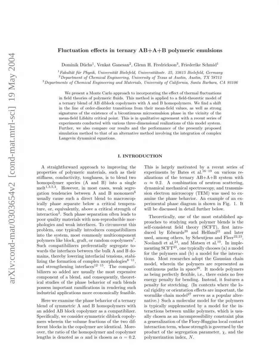
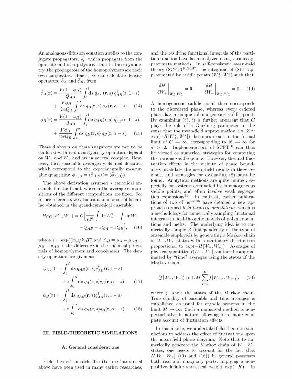
This is largely motivated by a recent series ofexperiments by Bates et al.16–19 on various re-alizations of the ternary AB+A+B system withα ≈ 0.2. A combination of neutron scattering,dynamical mechanical spectroscopy, and transmis-sion electron microscopy (TEM) was used to ex-amine the phase behavior. An example of an ex-perimental phase diagram is shown in Fig. 1. Itwill be discussed in detail further below.
Theoretically, one of the most established ap-proaches to studying such polymer blends is theself-consistent field theory (SCFT), first intro-duced by Edwards20 and Helfand21 and laterused, among others, by Scheutjens and Fleer22,23,Noolandi et al.24, and Matsen et al.10. In imple-menting SCFT25, one typically chooses (a) a modelfor the polymers and (b) a model for the interac-tions. Most researches adopt the Gaussian chainmodel, wherein the polymers are represented ascontinuous paths in space26. It models polymersas being perfectly flexible, i.e., there exists no freeenergy penalty for bending. Instead, it features apenalty for stretching. (In contexts where the lo-cal rigidity or orientation effects are important, thewormlike chain model27 serves as a popular alter-native.) Such a molecular model for the polymersis typically supplemented by a model for the in-teractions between unlike polymers, which is usu-ally chosen as an incompressibility constraint plusa generalization of the Flory-Huggins local contactinteraction term, whose strength is governed by theproduct of the segregation parameter, χ, and thepolymerization index, N .
FIG. 1. Experimental phase diagram19 of aPDMS-PEE/PDMS/PEE blend with α ≈ 0.2. Repro-duced by permission of The Royal Society of Chem-istry.
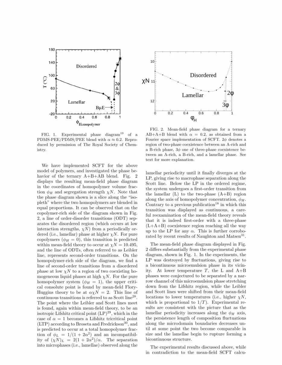
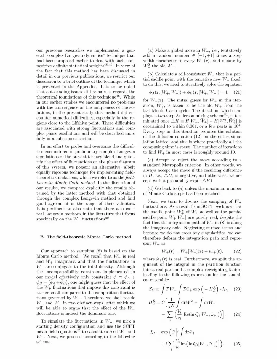
We have implemented SCFT for the abovemodel of polymers, and investigated the phase be-havior of the ternary A+B+AB blend. Fig. 2displays the resulting mean-field phase diagramin the coordinates of homopolymer volume frac-tion φH and segregation strength χN . Note thatthe phase diagram shown is a slice along the “iso-pleth” where the two homopolymers are blended inequal proportions. It can be observed that on thecopolymer-rich side of the diagram shown in Fig.2, a line of order-disorder transitions (ODT) sep-arates the disordered region (which occurs at lowinteraction strengths, χN) from a periodically or-dered (i.e., lamellar) phase at higher χN . For purecopolymers (φH = 0), this transition is predictedwithin mean-field theory to occur at χN = 10.495,and the line of ODTs, often referred to as Leiblerline, represents second-order transitions. On thehomopolymer-rich side of the diagram, we find aline of second-order transitions from a disorderedphase at low χN to a region of two coexisting ho-mogeneous liquid phases at high χN . For the purehomopolymer system (φH = 1), the upper criti-cal consolute point is found by mean-field Flory-Huggins theory to be at αχN = 2. This line ofcontinuous transitions is referred to as Scott line28.The point where the Leibler and Scott lines meetis found, again within mean-field theory, to be anisotropic Lifshitz critical point (LP)29, which in thecase of α = 1 becomes a Lifshitz tricritical point(LTP) according to Broseta and Fredrickson30, andis predicted to occur at a total homopolymer frac-tion of φL = 1/(1 + 2α2) and an incompatibil-ity of (χN)L = 2(1 + 2α2)/α. The separationinto microphases (i.e., lamellae) observed along the
Leibler line displays a steady increase in the
0 0.2 0.4 0.6 0.8 1φH
10
11
12
χΝDisordered
Lamellar 2φ
3φ
FIG. 2. Mean-field phase diagram for a ternaryAB+A+B blend with α = 0.2, as obtained from aFourier space implementation of SCFT. 2φ denotes aregion of two-phase coexistence between an A-rich anda B-rich phase, 3φ one of three-phase coexistence be-tween an A-rich, a B-rich, and a lamellar phase. Seetext for more explanation.
lamellar periodicity until it finally diverges at theLP, giving rise to macrophase separation along theScott line. Below the LP in the ordered regime,the system undergoes a first-order transition fromthe lamellar (L) to the two-phase (A+B) regionalong the axis of homopolymer concentration, φH .Contrary to a previous publication18 in which thistransition was displayed as continuous, a care-ful reexamination of the mean-field theory revealsthat it is indeed first-order with a three-phase(L+A+B) coexistence region reaching all the wayup to the LP for any α. This is further corrobo-rated by recent results of Naughton and Matsen31.
The mean-field phase diagram displayed in Fig.2 differs substantially from the experimental phasediagram, shown in Fig. 1. In the experiments, theLP was destroyed by fluctuations, giving rise toa bicontinuous microemulsion phase in its vicin-ity. At lower temperature T , the L and A+Bphases were conjectured to be separated by a nar-row channel of this microemulsion phase stretchingdown from the Lifshitz region, while the Leiblerand Scott lines were shifted from their mean-fieldlocations to lower temperatures (i.e., higher χN ,which is proportional to 1/T ). Experimental re-sults are consistent with the picture that as thelamellar periodicity increases along the φH axis,the persistence length of composition fluctuationsalong the microdomain boundaries decreases un-til at some point the two become comparable insize and the lamellae begin to rupture forming abicontinuous structure.
The experimental results discussed above, whilein contradiction to the mean-field SCFT calcu-
2
lations, are not entirely surprising when viewedin the context of theoretical studies pertaining tothe effect of fluctuations on the mean-field phasediagrams. Indeed, even in the context of thepure diblock copolymer (i.e. φH = 0), Leibler32
speculated that the order-disorder transition (pre-dicted to be second order within the mean-fieldtheory) would become a weakly first-order transi-tion when the effects of fluctuations are accountedfor. Such a reasoning was confirmed quantitativelyby Fredrickson and Helfand33, who extended anearlier analysis by Brazovskii34 to show that fluc-tuations change the order of the transition and alsoshift the transition to higher incompatibilities, χN .Further, they quantified such shifts in terms of aparameter that depends on the polymer density(or, equivalently in the context of a polymer melt,their molecular mass N). This parameter, denotedgenerically as C in this text, acts as a Ginzburgparameter35, and in the limit C → ∞, the mean-field solution is recovered.
The present study is motivated by the hypoth-esis that the fluctuation effects not accounted forwithin SCFT are responsible for the discrepanciesnoted between the experimental results and thetheoretical predictions for the ternary-blend phasebehavior. As a partial confirmation of our hypoth-esis, the experimental phase diagrams (Fig. 1) ofBates and co-workers deviate most clearly fromthe mean-field diagram for the PEE/PDMS/PEE-PDMS system, in situations where the molecularweights were much lower than in the other systems(i.e., where the C parameter is small). This arti-cle presents a theoretical examination of the effectof thermal fluctuations upon the phase behaviorof ternary blends. Our primary goal is to under-stand and quantify the shift in both the Leibler andScott lines and to examine the formation of the mi-croemulsion phases in such systems. Bicontinuousstructures such as the ones observed in the aboveexperiments are particularly interesting from anapplication point of view in that they are able toimpart many useful properties on polymer alloys.For example, if one blend component is conductingor gas-permeable, these properties will be passedon to the entire alloy. Also, mechanical proper-ties such as the strain at break and the toughnessindex have been observed to exhibit maxima withco-continuous structures36.
Previous simulation studies of fluctuation ef-fects in ternary diblock copolymer / homopoly-mer blends37,38,41,39,40, have mostly focused on theα = 1 case. Within a lattice polymer model,Muller and Schick37 have investigated the phase di-agram of a corresponding symmetrical A+B+ABblend. According to their results, the disorderedphase extends to higher χN than predicted by the
mean field theory, and the LTP is replaced by aregular tricritical point. Due to finite size effects,the transition to the lamellar phase could not belocalized quantitatively.
Particle-based models have the disadvantagethat one is restricted to studying relatively shortpolymers. This motivates the use of field theo-ries in simulations. Kielhorn and Muthukumar41
have studied the phase separation dynamics in thevicinity of the LTP within a Ginzburg-Landau freeenergy functional, which they derived from the Ed-wards model20 within the random phase approxi-mation (RPA), in the spirit of the theories for purediblock copolymer systems mentioned earlier32,33.Naively, one should expect that such a descriptionis adequate in the weak segregation limit, wherethe correlation length for composition fluctuationsis large. However, Kudlay and Stepanow42 have re-cently questioned this assumption. They pointedout that the fluctuations in RPA-derived Hamilto-nians have significant short wavelength contribu-tions which cannot be eliminated by renormaliza-tion and may lead to unphysical predictions.
In this work, we propose an alternative field-theoretic approach which rests directly on the Ed-wards model, without resorting to the additionalRPA approximation. The partition function isevaluated with a Monte Carlo algorithm. A re-lated algorithm, the complex Langevin method,has been presented recently by two of us43–45.Here we study two-dimensional ternary blends atα = 0.2 with both methods and compare the re-sults.
The remainder of this article is organized as fol-lows. In section II, we outline the field-theoreticformulation of our model. The simulation methodis presented in section III. In section IV, wepresent and discuss our results before we concludein section V with a summary and an outlook onfuture work.
II. THE FIELD-THEORETIC MODEL
In this section, we present a field-theoretic modelfor the system under consideration. To this effect,we consider a mixture of nA homopolymers of typeA, nB homopolymers of type B, and nAB symmet-ric block copolymers in a volume V . The polymer-ization index of the copolymer is denoted N , andthe corresponding quantities for the homopolymersare denoted NA = NB = αN . All chains are as-sumed to be monodisperse. We consider the caseof symmetric copolymers, where the fraction of Amonomers in the copolymer is f = 1/2. We re-
3
strict our attention to the concentration isopleth,where the homopolymers have equal volume frac-tions φHA = φHB = φH/2. The monomeric vol-umes of both A and B segments are assumed tobe identically equal to 1/ρ0. In this notation, theincompressibility constraint requires
nA = nB =φHρ0V
2αN; nAB = (1 − φH)
ρ0V
N, (1)
where V denotes the volume of the system. In theGaussian chain model, the segments are assumedto be perfectly flexible and are assigned a commonstatistical segment length b. The polymers are rep-resented as continuous space curves, Ri
j(s), wherei denotes the polymer species (A, B, or AB), jthe different polymers of a component, and s rep-resents the chain length variable measured alongthe chain backbone such that 0 ≤ s ≤ νj withνAB = 1 and νA = νB = α. Conformations of non-interacting polymers are given a Gaussian statisti-cal weight, exp(−H0), with a harmonic stretchingenergy given by (units of kBT ),
H0[R] =3
2Nb2
∑
i
nj∑
j=1
∫ νi
0
ds
∣
∣
∣
∣
dRij(s)
ds
∣
∣
∣
∣
2
. (2)
where bA = bB = bAB ≡ b is the statistical seg-ment length. Interactions between A and B seg-ments are modeled as local contact interactions bya pseudopotential with a Flory-Huggins quadraticform in the microscopic volume fractions,
HI [R] = χρ0
∫
dr φA(r)φB(r) (3)
which with the substitutions m = φB − φA, φ =
φA + φB transforms into
HI [R] =χρ0
4
∫
dr (φ2 − m2). (4)
χ denotes the Flory-Huggins parameter, and the
microscopic density operators φA and φB are de-fined by
φA(r) =N
ρ0
nAB∑
j=1
∫ f
0
ds δ(r − RABj (s))
+N
ρ0
nA∑
j=1
∫ α
0
ds δ(r − RAj (s)) (5)
φB(r) =N
ρ0
nAB∑
j=1
∫ 1
f
ds δ(r − RABj (s))
+N
ρ0
nB∑
j=1
∫ α
0
ds δ(r − RBj (s)). (6)
Furthermore, the incompressibility constraint isimplemented by the insertion of a Dirac delta func-tional46, and we obtain the canonical partitionfunction of the blend, ZC :
ZC ∝∫
∏
i
∏
j
DRij(s) δ(φ− 1) exp(−H0 −HI),
(7)where the
∫
DR denote functional integrationsover chain conformations. Representing the deltafunctional in exponential form and employing aHubbard-Stratonovich transformation on the m2
term in (4), we obtain
ZC ∝∫
∞
DW−
∫
i∞
DW+ exp[−HC(W−,W+)]
(8)with
HC(W−,W+) = C[ 1
χN
∫
drW 2− −
∫
drW+
−V (1−φH) lnQAB − V φH2α
(lnQA + lnQB)]
(9)
C =ρ0
NRdg0 . (10)
Here and throughout this article, all lengths are ex-pressed in units of the unperturbed radius of gyra-tion, Rg0 = b(N/(2d))1/2, where d is the space di-mension. The parameter C in the above equations,which occurs as a global prefactor to HC , acts as aGinzburg parameter such that in the limit C → ∞the partition function (8) is dominated by its sad-dle point and the mean-field solution becomes ex-act. In (9), i ≡
√−1, and QA, QB, and QAB de-
note respectively the single-chain partition func-tions for the A, B, and AB chains, in the potentialfields W−(r) and W+(r). Note that W− is conju-gate to the difference in A and B densities, m, and
W+ to the total density, φ. Moreover, W− is real,whereas W+ is imaginary, thereby rendering HC
complex.
The single-chain partition functions can be ex-pressed in terms of the Feynman-Kac formulae21
as:
Qi =
∫
dr qi(r, νi), (11)
where the propagators qi satisfy the diffusion equa-tions
∂
∂sqi(r, s) = △qi(r, s) − qiUi; qi(r, 0) = 1 (12)
UA = W+ −W−, 0 ≤ s ≤ α
UB = W+ +W−, 0 ≤ s ≤ α
UAB =
{
UA, 0 ≤ s < f
UB, f ≤ s ≤ 1
(13)
4
An analogous diffusion equation applies to the con-
jugate propagators, q†i , which propagate from theopposite end of a polymer. Due to their symme-try, the propagators of the homopolymers are theirown conjugates. Hence, we can calculate densityoperators, φA and φB , from
φA(r) =V (1 − φH)
QAB
∫ f
0
ds qAB(r, s) q†AB(r, 1−s)
+V φH2αQA
∫ α
0
ds qA(r, s) qA(r, α− s), (14)
φB(r) =V (1 − φH)
QAB
∫ 1
f
ds qAB(r, s) q†AB(r, 1−s)
+V φH2αQB
∫ α
0
ds qB(r, s) qB(r, α − s). (15)
These d shown on these snapshots are not to beconfused with real densityensity operators dependon W− and W+ and are in general complex. How-ever, their ensemble averages yield real densitieswhich correspond to the experimentally measur-
able quantities: φA,B = 〈φA,B〉(= 〈φA,B〉).The above derivation assumed a canonical en-
semble for the blend, wherein the average compo-sitions of the different compositions are fixed. Forfuture reference, we also list a similar set of formu-lae obtained in the grand-canonical ensemble:
HGC(W−,W+) = C[ 1
χN
∫
drW 2− −
∫
drW+
−QAB − zQA − zQB
]
, (16)
where z = exp((△µ/kBT ),and △µ ≡ µA − µAB =µB − µAB is the difference in the chemical poten-tials of homopolymers and copolymers. The den-sity operators are given as:
φA(r) :=
∫ f
0
ds qAB(r, s)q†AB(r, 1 − s)
+z
∫ α
0
ds qA(r, s)qA(r, α− s), (17)
φB(r) :=
∫ 1
f
ds qAB(r, s)q†AB(r, 1 − s)
+z
∫ α
0
ds qB(r, s)qB(r, α− s). (18)
III. FIELD-THEORETIC SIMULATIONS
A. General considerations
Field-theoretic models like the one introducedabove have been used in many earlier researches,
and the resulting functional integrals of the parti-tion function have been analyzed using various ap-proximate methods. In self-consistent mean-fieldtheory (SCFT)10,25,47, the integrand of (8) is ap-proximated by saddle points (W ∗
+,W∗−) such that
δH
δW+
∣
∣
∣
∣
W∗
+,W∗
−
= 0,δH
δW−
∣
∣
∣
∣
W∗
+,W∗
−
= 0. (19)
A homogeneous saddle point then correspondsto the disordered phase, whereas every orderedphase has a unique inhomogeneous saddle point.By examining (8), it is further apparent that Cplays the role of a Ginzburg parameter in thesense that the mean-field approximation, i.e. Z ≃exp(−H [W ∗
+,W∗−]), becomes exact in the formal
limit of C → ∞, corresponding to N → ∞ ford > 2. Implementations of SCFT10 can thusbe viewed as numerical strategies for computingthe various saddle points. However, thermal fluc-tuation effects in the vicinity of phase bound-aries invalidate the mean-field results in these re-gions, and strategies for evaluating (8) must befound. Analytical methods are quite limited, es-pecially for systems dominated by inhomogeneoussaddle points, and often involve weak segrega-tion expansions34. In contrast, earlier publica-tions of two of us43–45 have detailed a new ap-proach termed field-theoretic simulations, which isa methodology for numerically sampling functionalintegrals in field-theoretic models of polymer solu-tions and melts. The underlying idea is to nu-merically sample Z (independently of the type ofensemble employed) by generating a Markov chainof W−,W+ states with a stationary distributionproportional to exp(−H [W−,W+]). Averages ofphysical quantities f [W−,W+] can then be approx-imated by “time” averages using the states of theMarkov chain,
〈f [W−,W+]〉 ≈ 1/M
M∑
j=1
f [W−,j ,W+,j ], (20)
where j labels the states of the Markov chain.True equality of ensemble and time averages isestablished as usual for ergodic systems in thelimit M → ∞. Such a numerical method is non-perturbative in nature, allowing for a more com-plete account of fluctuation effects.
In this article, we undertake field-theoretic sim-ulations to address the effect of fluctuations uponthe mean-field phase diagram. Note that to nu-merically generate the Markov chain of W−,W+
states, one needs to account for the fact thatH [W−,W+] ((9) and (16)) in general possessesboth real and imaginary parts, implying a non-positive-definite statistical weight exp(−H). In
5
our previous researches we implemented a gen-eral “complex Langevin dynamics” technique thathad been proposed earlier to deal with such non-positive-definite statistical weights48,49. In view ofthe fact that this method has been discussed indetail in our previous publications, we restrict ourdiscussion to a brief outline of the technique whichis presented in the Appendix. It is to be notedthat outstanding issues still remain as regards thetheoretical foundations of this technique48. Whilein our earlier studies we encountered no problemswith the convergence or the uniqueness of the so-lutions, in the present study this method did en-counter numerical difficulties, especially in the re-gions close to the Lifshitz point. These difficultiesare associated with strong fluctuations and com-plex phase oscillations and will be described morefully in a subsequent section.
In an effort to probe and overcome the difficul-ties encountered in preliminary complex Langevinsimulations of the present ternary blend and quan-tify the effect of fluctuations on the phase diagramof this system, we present an alternative, albeitequally rigorous technique for implementing field-theoretic simulations, which we refer to as the field-
theoretic Monte Carlo method. In the discussion ofour results, we compare explicitly the results ob-tained by the latter method with that obtainedthrough the complex Langevin method and findgood agreement in the range of their validities.It is pertinent to also note that there also existreal Langevin methods in the literature that focusspecifically on the W− fluctuations50.
B. The field-theoretic Monte Carlo method
Our approach to sampling (8) is based on theMonte Carlo method. We recall that W− is realand W+ imaginary, and that the fluctuations inW+ are conjugate to the total density. Althoughthe incompressibility constraint implemented inour model effectively only constrains φ ≡ φA +φB = 〈φA+ φB〉, one might guess that the effect ofthe W+ fluctuations that impose this constraint israther small compared to the composition fluctua-tions governed by W−. Therefore, we shall tackleW− and W+ in two distinct steps, after which wewill be able to argue that the effect of the W−
fluctuations is indeed the dominant one.
To simulate the fluctuations in W−, we pick astarting density configuration and use the SCFTmean-field equations25 to calculate a seed W− andW+. Next, we proceed according to the followingscheme:
(a) Make a global move in W−, i.e., tentativelyadd a random number ∈ [−1,+1] times a stepwidth parameter to every W−(r), and denote byW 0
− the old W−.
(b) Calculate a self-consistent W+ that is a par-tial saddle point with the tentative new W− fixed;to do this, we need to iteratively solve the equation
φA(r; [W+,W−]) + φB(r; [W+,W−]) = 1 (21)
for W+(r). The initial guess for W+ in this iter-ation, W 0
+, is taken to be the old W+ from thelast Monte Carlo cycle. The iteration, which em-ploys a two-step Anderson mixing scheme51, is ter-minated once △H ≡ H [W−, W+] −H [W 0
−, W0+] is
determined to within 0.001, or a few parts in 104.Every step in this iteration requires the solutionof the diffusion equation (12) on the entire simu-lation lattice, and this is where practically all thecomputing time is spent. The number of iterationsto find W+ in most cases is roughly around 10.
(c) Accept or reject the move according to astandard Metropolis criterion. In other words, wealways accept the move if the resulting differencein H , i.e., △H , is negative, and otherwise, we ac-cept with a probability exp(−△H).
(d) Go back to (a) unless the maximum numberof Monte Carlo steps has been reached.
Next, we turn to discuss the sampling of W+
fluctuations. As a result from SCFT, we know thatthe saddle point W ∗
+ of W+ as well as the partial
saddle point W+[W−] are purely real, despite thefact that the integration path of W+ in (8) is alongthe imaginary axis. Neglecting surface terms andbecause we do not cross any singularities, we cantherefore deform the integration path and repre-sent W+ as
W+(r) = W+[W−](r) + iω+(r), (22)
where ω+(r) is real. Furthermore, we split the ar-gument of the integral in the partition functioninto a real part and a complex reweighting factor,leading to the following expression for the canoni-cal ensemble:
ZC ∝∫
DW−
∫
Dω+ exp(
−HRC
)
· IC , (23)
HRC = C
[ 1
χN
∫
drW 2− −
∫
drW+
−∑
i
(Viνi
Re(lnQi[W−, ω+]))]
, (24)
IC = exp(
C[
i
∫
drω+
+ i∑
i
Viνi
Im(
lnQi[W−, ω+])
])
. (25)
6
where Vi is the volume occupied by species i. Inthe grand canonical ensemble the correspondingexpression is:
ZGC ∝∫
DW−
∫
Dω+ exp(
−HRGC
)
· IGC , (26)
HRGC = C
[ 1
χN
∫
drW 2− −
∫
drW+
−∑
i
zi Re(
Qi[W−, ω+]))
]
, (27)
IGC = exp(
C[
i
∫
drω+
+ i∑
i
zi Im(
Qi[W−, ω+])
])
, (28)
where zAB = 1 and zA = zB = z.
We can thus in principle simulate both W− andW+ fluctuations, e.g., by alternating a move inW− with a number of moves in ω+ and replacing△HC,GC with △HR
C,GC in the Metropolis criterion.Each configuration then needs to be weighted withthe factor IC,GC for the purpose of computing av-erages. We note that the propagators and the fieldterm in the diffusion equation (12) are now com-plex, but the averages of all physical quantities willapproach real values in equilibrium.
At this point, a remark concerning our numericalmethods is due: the single most time-consumingpart in doing our simulations is the solution ofthe diffusion equation (12). Initially, we used ei-ther the Crank-Nicholson (CN) or DuFort-Frankel(DF) finite differencing schemes52,53 to effectuatethis task. As it turned out, however, a pseudo-spectral method that had been used successfullyin the past to solve the mathematically very sim-ilar Schrodinger equation and that had recentlybeen applied to SCFT54,55 was far better suitedfor our needs. Typically, it allowed for an order ofmagnitude higher values of contour step ds thaneither CN or DF to achieve the same accuracy.Implementing the scheme with highly optimizedFast Fourier Transform routines like the publiclyavailable FFTW library56, the computing time percontour step is only roughly double that needed forDF and half that needed for CN on a single pro-cessor. We therefore regard it as the method ofchoice in the context of polymer field theory. Forthe larger system sizes to be discussed in the nextsection, a parallel version of the code was used.
C. Analysis of W+ fluctuations
Evidently, the W+ fluctuations exert their influ-ence on the simulation in two ways: (a) through
the complex reweighting factor IC or IGC and (b)through the difference of △HR from △H .
We consider first IGC and to this end split thecomplex diffusion equation into two real equationsfor the real and imaginary parts of the propagatorfor polymers of type i, denoted qRi and qIi , respec-tively. Note the symmetry properties of this cou-pled set of equations with respect to a sign changein ω+: for W+ = W+ ± iω+ we obtain
∂∂sq
Ri = △qRi − Uiq
Ri ± ω+q
Ii ,
± ∂∂sq
Ii = ± △qIi ∓ Uiq
Ii − ω+q
Ri .
(29)
We see that qRi remains unchanged whereas qIi goesto −qIi . Thus, for the corresponding single-chainpartition function Qi = QRi + iQIi , Q
Ri is symmet-
ric in ω+, and QIi antisymmetric. Furthermore,the exponent of the reweighting factor IGC is anti-symmetric in ω+ (cf. (28)). Since in the partitionfunction (26) we integrate over all possible config-urations of ω+, the imaginary parts of IGC cancelout for each antisymmetric pair, and consequently,we effectively only need to apply the real part ofIGC :
IRGC = cos
(
C
[
∫
drω+ +∑
i
ziQIi [W−, ω+]
])
.
(30)
These symmetries reveal that in a functionalexpansion of Qi in ω+ around the partial saddlepoint, Qi[W−], the even-order terms coincide withthe expansion of QRi , and the odd-order terms withthat of QIi . Moreover,
δQiδW+
≡ δQIiδω+
, (31)
and
∑
i
ziδQIiδω+
=∑
i
ziδQiδW+
= −〈ρ〉 = −1 (32)
by virtue of the incompressibility constraint.Hence,
∑
i
ziQIi = −
∫
drω+ + O(ω3+), (33)
and finally
IGC = cos(
O(ω3+))
= 1 −O(ω6+), (34)
QRi = Qi[W−] + O(ω2+). (35)
Based on these analytical results, we should ex-pect IGC to deviate only very slightly from unityso that it can be neglected in most practical cases.
7
Hence, the impact of the W+ fluctuations wouldmaterialize solely as a (real) O(ω2
+) contribution toHGC . The above derivation of (34) and (35) wasfor the grand canonical ensemble but holds true ifone is to derive analogous relations in the canon-ical ensemble, as well, because the leading termof lnQi is linear in ω+, as in the grand canon-ical ensemble. It should however be noted thatin the canonical ensemble, the gauge invariance ofthe theory to a constant shift of the ω+ field al-lows the introduction of a spurious phase factoreiψ that preserves HC (and hence |Qi| and HR).This ψ field will freely move in canonical simula-tions unless constrained, e.g., by demanding that∫
drω+(r) = 0. In contrast, in the grand canonicalensemble, QR and hence HR are to lowest approx-imation quadratic functions around ω+ = 0. As aresult the shape of the HR(W+) energy landscapeis much steeper in the grand canonical ensemblethan in the canonical, and no constraint is needed.
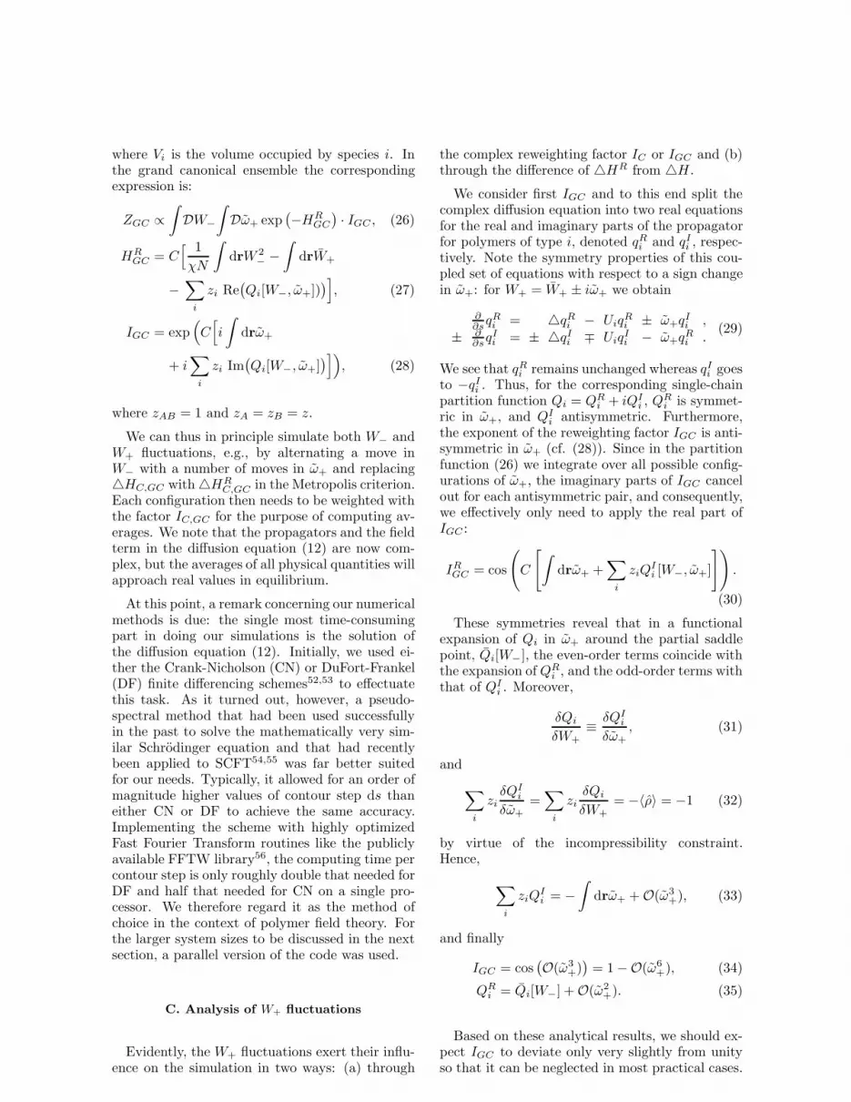
While the above considerations can only give usan indication of the insignificance of the W+ fluc-tuations, we have also done test simulations to getmore conclusive estimates. We therefore choosethe grand canonical ensemble for testing our simu-lation technique of W+ fluctuations. Before start-ing a run at z = 2, χN = 12, α = 0.2, and C = 50,we fully equilibrated a simulation of W− fluctua-tions only with the same parameters, which startedfrom a disordered configuration and ran a millionMonte Carlo steps. This set of parameters is veryclose to the (fluctuation-corrected) order-disordertransition in the phase diagram, on the disorderedside. The average homopolymer fraction, φH , is0.65. On a 32×32 lattice with periodic boundaryconditions, we used dx = 0.78125. We then tookthis equilibrated configuration and switched on theW+ fluctuations, again making ten (global) movesin W+ after each move in W− so as to roughlyspend equal amounts of computing time for thetwo types of moves. Note in Fig. 3 how HGC
quickly increases and then plateaus off, indicatingthat the W+ fluctuations have become saturated.
For the same run, we recorded the quantity△H∗ = △HR − △H (cf. Eqs. (24) and (27)),which is displayed in the inset of Fig. 3. One caninterpret
√
〈(△H∗)2〉 as a measure for the devi-ation of the simulation from a reference case inwhich only W− fluctuations are simulated. Thissimulation was done with a chain-contour dis-cretization of ds = 0.01, which allows for thecalculation of △H to within 0.01. Typically, insimulations involving the W− field alone, we usedds = 0.05 in order to save computing time. Thediscretization error of △H in this case is increasedto <∼ 0.08. Considering that typical values of △Hare on the order of ±3, this appears like a very
0 20000 40000−0.1
−0.05
0
0.05
0.1
∆H*
0 20000 40000MCS
0
100
200
300
400
500
600
700
Re(
H)
FIG. 3. Re(H) in a simulation of W− and W+ vs.number of Monte Carlo steps in W− for C = 50,χN = 12, z = 2 (grand canonical ensemble), startedfrom a configuration equilibrated in W−. Each W−
step alternates with ten steps in ω+. Inset shows △H∗
(difference of △H and a reference value at ω+ fluctua-tions switched off) in the same simulation.
moderate numerical error. At the same time, werealize that the effect of the fluctuations in W+
expressed through △H∗ is well below our stan-dard numerical accuracy:
√
〈(△H∗)2〉 ≈ 0.022.Furthermore, the average of △H∗ very closely ap-proximates zero, so there is no drift of △H as aresult. We therefore conclude that contributionsof the W+ fluctuations to HR cannot be distin-guished as such from numerical inaccuracies.
Next, we examine the reweighting factor, IGC ,in the particular simulation discussed above. Nu-merically, we must evaluate:
IRGC = cos
(
C
[
∫
drω+ +∑
i
ziQIi
])
≡ cos(A)
(36)
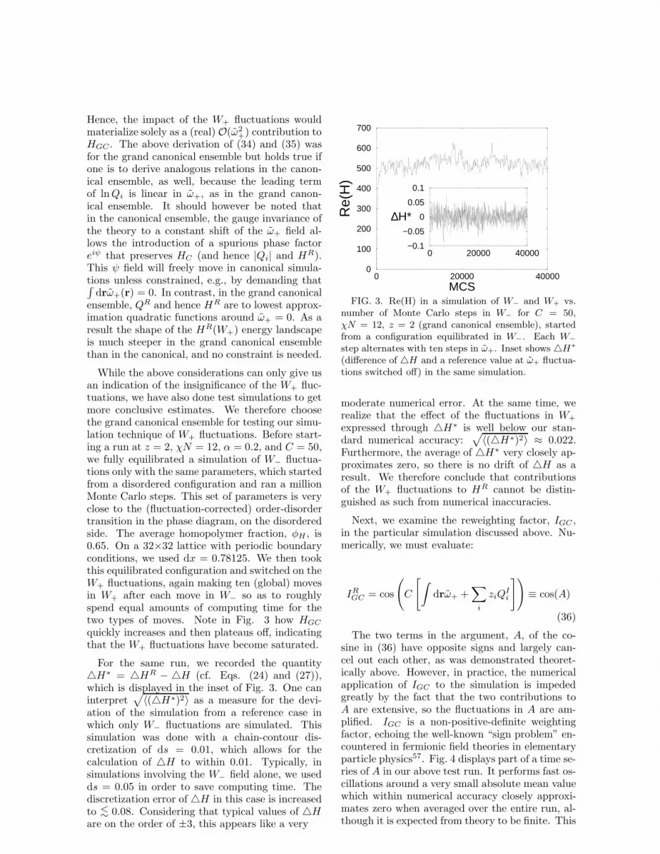
The two terms in the argument, A, of the co-sine in (36) have opposite signs and largely can-cel out each other, as was demonstrated theoret-ically above. However, in practice, the numericalapplication of IGC to the simulation is impededgreatly by the fact that the two contributions toA are extensive, so the fluctuations in A are am-plified. IGC is a non-positive-definite weightingfactor, echoing the well-known “sign problem” en-countered in fermionic field theories in elementaryparticle physics57. Fig. 4 displays part of a time se-ries of A in our above test run. It performs fast os-cillations around a very small absolute mean valuewhich within numerical accuracy closely approxi-mates zero when averaged over the entire run, al-though it is expected from theory to be finite. This
8
0 1000 2000 3000 4000 5000MCS
-5
0
5
A
FIG. 4. The argument, A, of the cosine in thereweighting factor in the same simulation as in Fig. 3.
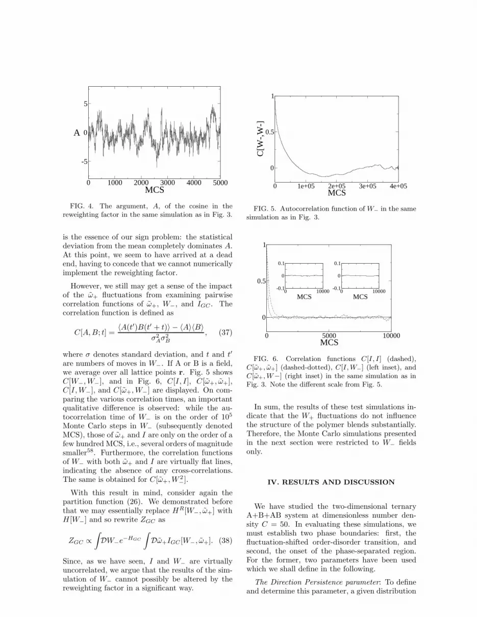
is the essence of our sign problem: the statisticaldeviation from the mean completely dominates A.At this point, we seem to have arrived at a deadend, having to concede that we cannot numericallyimplement the reweighting factor.
However, we still may get a sense of the impactof the ω+ fluctuations from examining pairwisecorrelation functions of ω+, W−, and IGC . Thecorrelation function is defined as
C[A,B; t] =〈A(t′)B(t′ + t)〉 − 〈A〉〈B〉
σ2Aσ
2B
, (37)
where σ denotes standard deviation, and t and t′
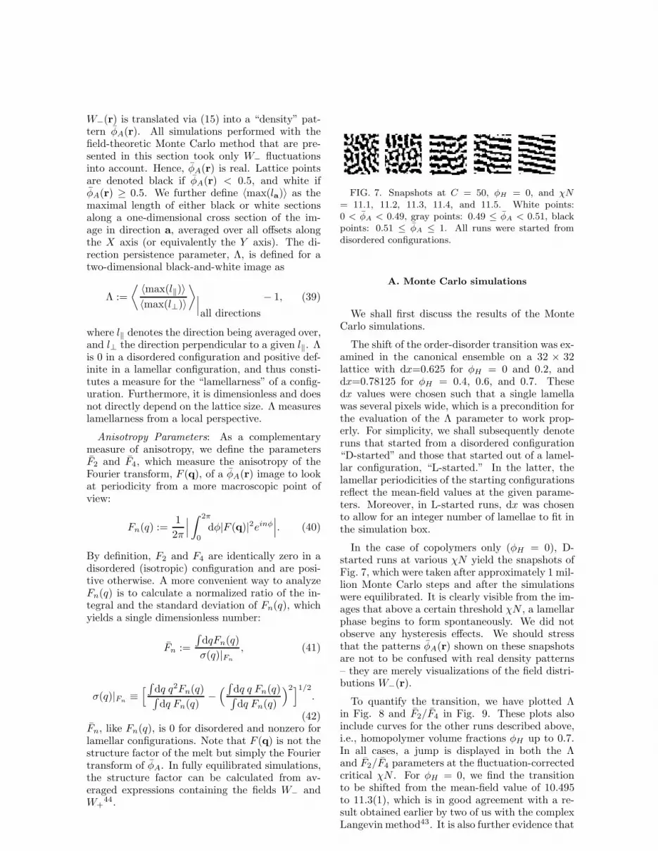
are numbers of moves in W−. If A or B is a field,we average over all lattice points r. Fig. 5 showsC[W−,W−], and in Fig. 6, C[I, I], C[ω+, ω+],C[I,W−], and C[ω+,W−] are displayed. On com-paring the various correlation times, an importantqualitative difference is observed: while the au-tocorrelation time of W− is on the order of 105
Monte Carlo steps in W− (subsequently denotedMCS), those of ω+ and I are only on the order of afew hundred MCS, i.e., several orders of magnitudesmaller58. Furthermore, the correlation functionsof W− with both ω+ and I are virtually flat lines,indicating the absence of any cross-correlations.The same is obtained for C[ω+,W
2−].
With this result in mind, consider again thepartition function (26). We demonstrated beforethat we may essentially replace HR[W−, ω+] withH [W−] and so rewrite ZGC as
ZGC ∝∫
DW−e−HGC
∫
Dω+IGC [W−, ω+]. (38)
Since, as we have seen, I and W− are virtuallyuncorrelated, we argue that the results of the sim-ulation of W− cannot possibly be altered by thereweighting factor in a significant way.
0 1e+05 2e+05 3e+05 4e+05MCS
0
0.5
1
C[W
-,W
-]
FIG. 5. Autocorrelation function of W− in the samesimulation as in Fig. 3.
0 5000 10000MCS
0
0.5
1
0 10000MCS
-0.1
0
0.1
0 10000MCS
-0.1
0
0.1
FIG. 6. Correlation functions C[I, I ] (dashed),C[ω+, ω+] (dashed-dotted), C[I, W−] (left inset), andC[ω+, W−] (right inset) in the same simulation as inFig. 3. Note the different scale from Fig. 5.
In sum, the results of these test simulations in-dicate that the W+ fluctuations do not influencethe structure of the polymer blends substantially.Therefore, the Monte Carlo simulations presentedin the next section were restricted to W− fieldsonly.
IV. RESULTS AND DISCUSSION
We have studied the two-dimensional ternaryA+B+AB system at dimensionless number den-sity C = 50. In evaluating these simulations, wemust establish two phase boundaries: first, thefluctuation-shifted order-disorder transition, andsecond, the onset of the phase-separated region.For the former, two parameters have been usedwhich we shall define in the following.
The Direction Persistence parameter: To defineand determine this parameter, a given distribution
9
W−(r) is translated via (15) into a “density” pat-tern φA(r). All simulations performed with thefield-theoretic Monte Carlo method that are pre-sented in this section took only W− fluctuationsinto account. Hence, φA(r) is real. Lattice pointsare denoted black if φA(r) < 0.5, and white ifφA(r) ≥ 0.5. We further define 〈max(la)〉 as themaximal length of either black or white sectionsalong a one-dimensional cross section of the im-age in direction a, averaged over all offsets alongthe X axis (or equivalently the Y axis). The di-rection persistence parameter, Λ, is defined for atwo-dimensional black-and-white image as
Λ :=
⟨ 〈max(l‖)〉〈max(l⊥)〉
⟩
∣
∣
∣
all directions
− 1, (39)
where l‖ denotes the direction being averaged over,and l⊥ the direction perpendicular to a given l‖. Λis 0 in a disordered configuration and positive def-inite in a lamellar configuration, and thus consti-tutes a measure for the “lamellarness” of a config-uration. Furthermore, it is dimensionless and doesnot directly depend on the lattice size. Λ measureslamellarness from a local perspective.
Anisotropy Parameters: As a complementarymeasure of anisotropy, we define the parametersF2 and F4, which measure the anisotropy of theFourier transform, F (q), of a φA(r) image to lookat periodicity from a more macroscopic point ofview:
Fn(q) :=1
2π
∣
∣
∣
∫ 2π
0
dφ|F (q)|2einφ∣
∣
∣. (40)
By definition, F2 and F4 are identically zero in adisordered (isotropic) configuration and are posi-tive otherwise. A more convenient way to analyzeFn(q) is to calculate a normalized ratio of the in-tegral and the standard deviation of Fn(q), whichyields a single dimensionless number:
Fn :=
∫
dqFn(q)
σ(q)|Fn
, (41)
σ(q)|Fn≡[
∫
dq q2Fn(q)∫
dq Fn(q)−(
∫
dq q Fn(q)∫
dq Fn(q)
)2]1/2
.
(42)Fn, like Fn(q), is 0 for disordered and nonzero forlamellar configurations. Note that F (q) is not thestructure factor of the melt but simply the Fouriertransform of φA. In fully equilibrated simulations,the structure factor can be calculated from av-eraged expressions containing the fields W− andW+
44.
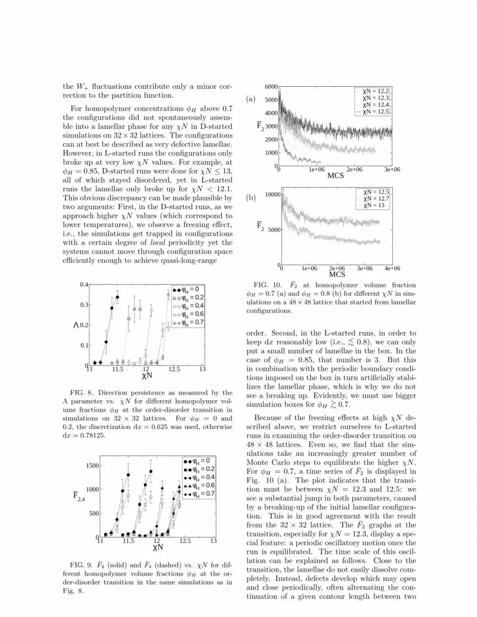
FIG. 7. Snapshots at C = 50, φH = 0, and χN
= 11.1, 11.2, 11.3, 11.4, and 11.5. White points:0 < φA < 0.49, gray points: 0.49 ≤ φA < 0.51, blackpoints: 0.51 ≤ φA ≤ 1. All runs were started fromdisordered configurations.
A. Monte Carlo simulations
We shall first discuss the results of the MonteCarlo simulations.
The shift of the order-disorder transition was ex-amined in the canonical ensemble on a 32 × 32lattice with dx=0.625 for φH = 0 and 0.2, anddx=0.78125 for φH = 0.4, 0.6, and 0.7. Thesedx values were chosen such that a single lamellawas several pixels wide, which is a precondition forthe evaluation of the Λ parameter to work prop-erly. For simplicity, we shall subsequently denoteruns that started from a disordered configuration“D-started” and those that started out of a lamel-lar configuration, “L-started.” In the latter, thelamellar periodicities of the starting configurationsreflect the mean-field values at the given parame-ters. Moreover, in L-started runs, dx was chosento allow for an integer number of lamellae to fit inthe simulation box.
In the case of copolymers only (φH = 0), D-started runs at various χN yield the snapshots ofFig. 7, which were taken after approximately 1 mil-lion Monte Carlo steps and after the simulationswere equilibrated. It is clearly visible from the im-ages that above a certain threshold χN , a lamellarphase begins to form spontaneously. We did notobserve any hysteresis effects. We should stressthat the patterns φA(r) shown on these snapshotsare not to be confused with real density patterns– they are merely visualizations of the field distri-butions W−(r).
To quantify the transition, we have plotted Λin Fig. 8 and F2/F4 in Fig. 9. These plots alsoinclude curves for the other runs described above,i.e., homopolymer volume fractions φH up to 0.7.In all cases, a jump is displayed in both the Λand F2/F4 parameters at the fluctuation-correctedcritical χN . For φH = 0, we find the transitionto be shifted from the mean-field value of 10.495to 11.3(1), which is in good agreement with a re-sult obtained earlier by two of us with the complexLangevin method43. It is also further evidence that
10
the W+ fluctuations contribute only a minor cor-rection to the partition function.
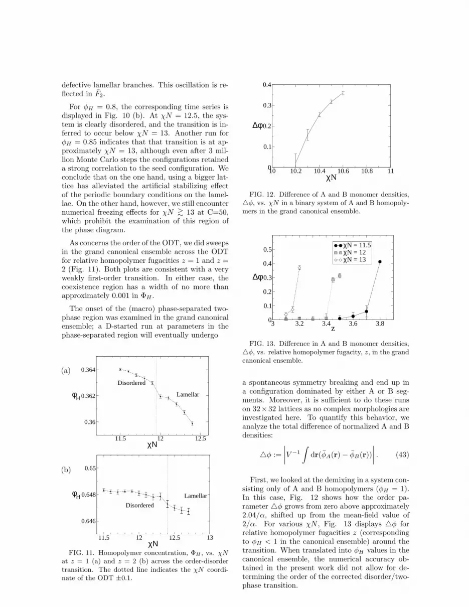
For homopolymer concentrations φH above 0.7the configurations did not spontaneously assem-ble into a lamellar phase for any χN in D-startedsimulations on 32×32 lattices. The configurationscan at best be described as very defective lamellae.However, in L-started runs the configurations onlybroke up at very low χN values. For example, atφH = 0.85, D-started runs were done for χN ≤ 13,all of which stayed disordered, yet in L-startedruns the lamellae only broke up for χN < 12.1.This obvious discrepancy can be made plausible bytwo arguments: First, in the D-started runs, as weapproach higher χN values (which correspond tolower temperatures), we observe a freezing effect,i.e., the simulations get trapped in configurationswith a certain degree of local periodicity yet thesystems cannot move through configuration spaceefficiently enough to achieve quasi-long-range
11 11.5 12 12.5 13χN
0
0.1
0.2
0.3
0.4
Λ
φΗ = 0φΗ = 0.2φΗ = 0.4φΗ = 0.6φΗ = 0.7
FIG. 8. Direction persistence as measured by theΛ parameter vs. χN for different homopolymer vol-ume fractions φH at the order-disorder transition insimulations on 32 × 32 lattices. For φH = 0 and0.2, the discretization dx = 0.625 was used, otherwisedx = 0.78125.
11 11.5 12 12.5 13χN
0
500
1000
1500
F2,4
φΗ = 0φΗ = 0.2φΗ = 0.4φΗ = 0.6φΗ = 0.7
FIG. 9. F2 (solid) and F4 (dashed) vs. χN for dif-ferent homopolymer volume fractions φH at the or-der-disorder transition in the same simulations as inFig. 8.
0 1e+06 2e+06 3e+06 4e+06MCS
0
5000
10000
F2
χN = 12.5χN = 12.7χN = 13
(b)
0 1e+06 2e+06 3e+06MCS
0
1000
2000
3000
4000
5000
6000
F2
χN = 12.2χN = 12.3χN = 12.4χN = 12.5
(a)
FIG. 10. F2 at homopolymer volume fractionφH = 0.7 (a) and φH = 0.8 (b) for different χN in sim-ulations on a 48× 48 lattice that started from lamellarconfigurations.
order. Second, in the L-started runs, in order tokeep dx reasonably low (i.e., <∼ 0.8), we can onlyput a small number of lamellae in the box. In thecase of φH = 0.85, that number is 3. But thisin combination with the periodic boundary condi-tions imposed on the box in turn artificially stabi-lizes the lamellar phase, which is why we do notsee a breaking up. Evidently, we must use biggersimulation boxes for φH >∼ 0.7.
Because of the freezing effects at high χN de-scribed above, we restrict ourselves to L-startedruns in examining the order-disorder transition on48 × 48 lattices. Even so, we find that the sim-ulations take an increasingly greater number ofMonte Carlo steps to equilibrate the higher χN .For φH = 0.7, a time series of F2 is displayed inFig. 10 (a). The plot indicates that the transi-tion must be between χN = 12.3 and 12.5: wesee a substantial jump in both parameters, causedby a breaking-up of the initial lamellar configura-tion. This is in good agreement with the resultfrom the 32 × 32 lattice. The F2 graphs at thetransition, especially for χN = 12.3, display a spe-cial feature: a periodic oscillatory motion once therun is equilibrated. The time scale of this oscil-lation can be explained as follows. Close to thetransition, the lamellae do not easily dissolve com-pletely. Instead, defects develop which may openand close periodically, often alternating the con-tinuation of a given contour length between two
11
defective lamellar branches. This oscillation is re-flected in F2.
For φH = 0.8, the corresponding time series isdisplayed in Fig. 10 (b). At χN = 12.5, the sys-tem is clearly disordered, and the transition is in-ferred to occur below χN = 13. Another run forφH = 0.85 indicates that that transition is at ap-proximately χN = 13, although even after 3 mil-lion Monte Carlo steps the configurations retaineda strong correlation to the seed configuration. Weconclude that on the one hand, using a bigger lat-tice has alleviated the artificial stabilizing effectof the periodic boundary conditions on the lamel-lae. On the other hand, however, we still encounternumerical freezing effects for χN >∼ 13 at C=50,which prohibit the examination of this region ofthe phase diagram.
As concerns the order of the ODT, we did sweepsin the grand canonical ensemble across the ODTfor relative homopolymer fugacities z = 1 and z =2 (Fig. 11). Both plots are consistent with a veryweakly first-order transition. In either case, thecoexistence region has a width of no more thanapproximately 0.001 in ΦH .
The onset of the (macro) phase-separated two-phase region was examined in the grand canonicalensemble; a D-started run at parameters in thephase-separated region will eventually undergo
11.5 12 12.5 13χΝ
0.646
0.648
0.65
φΗDisordered
Lamellar
(b)
11.5 12 12.5χΝ
0.36
0.362
0.364
φΗ
Disordered
Lamellar
(a)
FIG. 11. Homopolymer concentration, ΦH , vs. χN
at z = 1 (a) and z = 2 (b) across the order-disordertransition. The dotted line indicates the χN coordi-nate of the ODT ±0.1.
10 10.2 10.4 10.6 10.8 11χN
0
0.1
0.2
0.3
0.4
∆φ
FIG. 12. Difference of A and B monomer densities,△φ, vs. χN in a binary system of A and B homopoly-mers in the grand canonical ensemble.
3 3.2 3.4 3.6 3.8z
0
0.1
0.2
0.3
0.4
0.5
∆φ
χN = 11.5χN = 12χN = 13
FIG. 13. Difference in A and B monomer densities,△φ, vs. relative homopolymer fugacity, z, in the grandcanonical ensemble.
a spontaneous symmetry breaking and end up ina configuration dominated by either A or B seg-ments. Moreover, it is sufficient to do these runson 32×32 lattices as no complex morphologies areinvestigated here. To quantify this behavior, weanalyze the total difference of normalized A and Bdensities:
△φ :=
∣
∣
∣
∣
V −1
∫
dr(φA(r) − φB(r))
∣
∣
∣
∣
. (43)
First, we looked at the demixing in a system con-sisting only of A and B homopolymers (φH = 1).In this case, Fig. 12 shows how the order pa-rameter △φ grows from zero above approximately2.04/α, shifted up from the mean-field value of2/α. For various χN , Fig. 13 displays △φ forrelative homopolymer fugacities z (correspondingto φH < 1 in the canonical ensemble) around thetransition. When translated into φH values in thecanonical ensemble, the numerical accuracy ob-tained in the present work did not allow for de-termining the order of the corrected disorder/two-phase transition.
12
11 11.5 12 12.5 13χN
0
500
1000
1500
2000
F2,4
φΗ = 0φΗ = 0.2φΗ = 0.4φΗ = 0.6
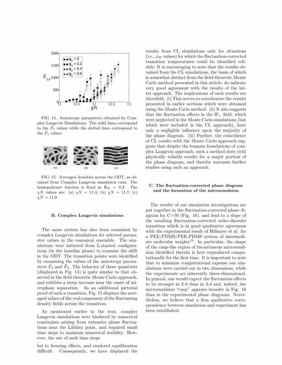
FIG. 14. Anisotropy parameters obtained by Com-plex Langevin Simulations. The solid lines correspondto the F2 values while the dotted lines correspond tothe F4 values.
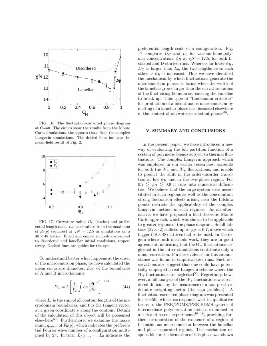
FIG. 15. Averaged densities across the ODT, as ob-tained from Complex Langevin simulation runs. Thehomopolymer fraction is fixed at ΦH = 0.2. TheχN values are: (a) χN = 11.4; (b) χN = 11.7; (c)χN = 11.9.
B. Complex Langevin simulations
The same system has also been examined bycomplex Langevin simulations for selected param-eter values in the canonical ensemble. The sim-ulations were initiated from L-started configura-tions (in the lamellar phase) to examine the shiftin the ODT. The transition points were identifiedby examining the values of the anisotropy param-eters F2 and F4. The behavior of these quantities(displayed in Fig. 14) is quite similar to that ob-served in the field-theoretic Monte Carlo approach,and exhibits a steep increase near the onset of mi-crophase separation. As an additional pictorialproof of such a transition, Fig. 15 displays the aver-aged values of the real component of the fluctuatingdensity fields across the transition.
As mentioned earlier in the text, complexLangevin simulations were hindered by numericalconstraints arising from extensive phase fluctua-tions near the Lifshitz point, and required smalltime steps to maintain numerical stability. How-ever, the use of such time steps
led to freezing effects, and rendered equilibrationdifficult. Consequently, we have displayed the
results from CL simulations only for situations(i.e., φH values) for which the fluctuation-correctedtransition temperatures could be identified reli-ably. It is encouraging to note that the results ob-tained from the CL simulations, the basis of whichis somewhat distinct from the field-theoretic MonteCarlo method presented in this article, do indicatevery good agreement with the results of the lat-ter approach. The implications of such results arethreefold: (i) This serves to corroborate the resultspresented in earlier sections which were obtainedusing the Monte Carlo method. (ii) It also suggeststhat the fluctuation effects in the W+ field, whichwere neglected in the Monte Carlo simulations (butwhich were included in the CL approach), haveonly a negligible influence upon the majority ofthe phase diagram. (iii) Further, the coincidenceof CL results with the Monte Carlo approach sug-gests that despite the tenuous foundations of com-plex Langevin approach, such a method does yieldphysically reliable results for a major portion ofthe phase diagram, and thereby warrants furtherstudies using such an approach.
C. The fluctuation-corrected phase diagram
and the formation of the microemulsion
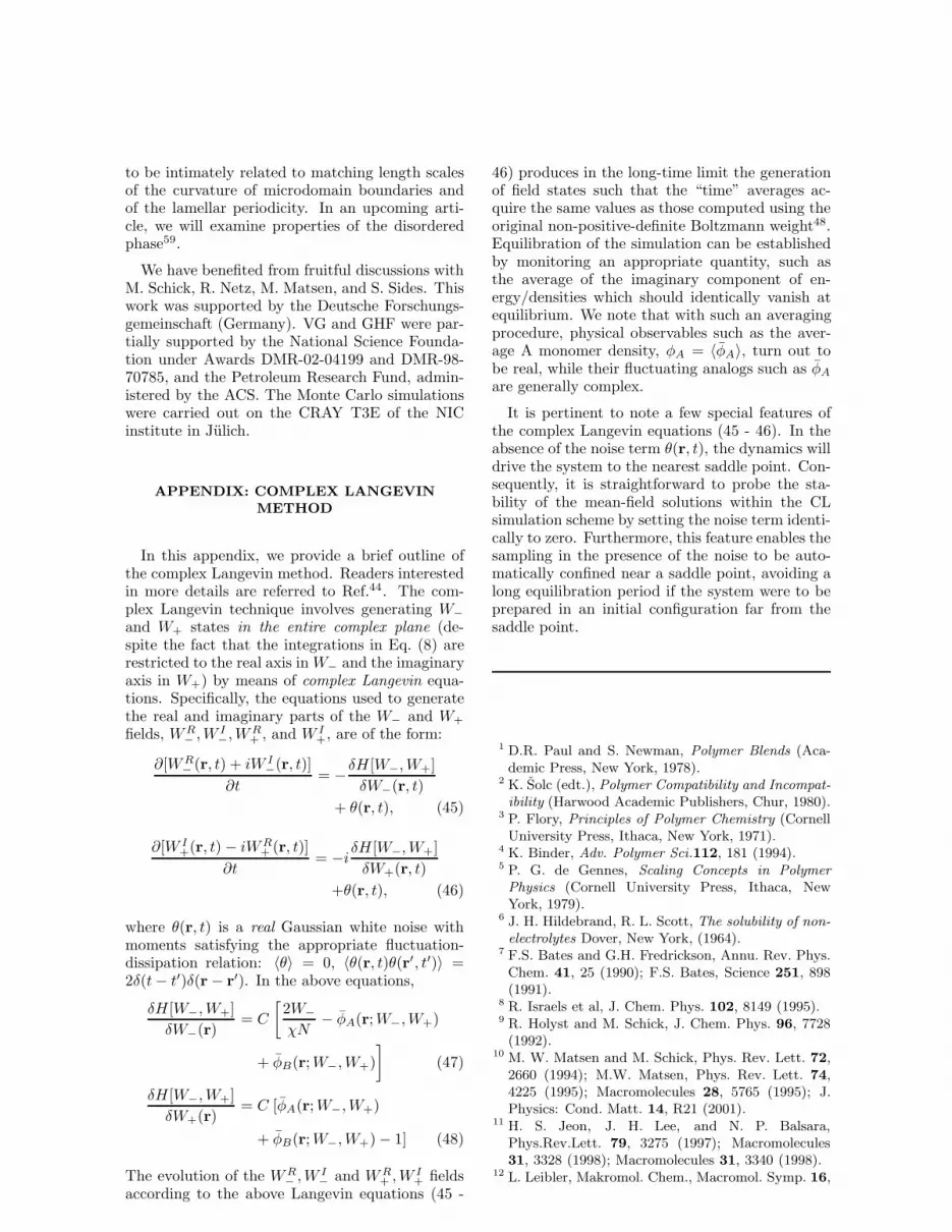
The results of our simulation investigations areput together in the fluctuation-corrected phase di-agram for C=50 (Fig. 16), and lead to a slope ofthe resulting fluctuation-corrected order-disordertransition which is in good qualitative agreementwith the experimental result of Hillmyer et al. fora PEE/PDMS/PEE-PDMS system of intermedi-ate molecular weights19. In particular, the shapeof the cusp-like region of bicontinuous microemul-sion identified therein is here reproduced compu-tationally for the first time. It is important to notethat to minimize computational expense our sim-ulations were carried out in two dimensions, whilethe experiments are inherently three-dimensional.In general, one would expect the fluctuation effectsto be stronger in 2-d than in 3-d and, indeed, themicroemulsion “cusp” appears broader in Fig. 16than in the experimental phase diagrams. Never-theless, we believe that a firm qualitative corre-spondence between simulation and experiment hasbeen established.
13
0 0.2 0.4 0.6 0.8 1φH
10
11
12
13
14
χΝDisordered
Lamellar
2φ
FIG. 16. The fluctuation-corrected phase diagramat C=50. The circles show the results from the MonteCarlo simulations, the squares those from the complexLangevin simulations. The dotted lines indicate themean-field result of Fig. 2.
0.7 0.8 0.9φ
H
4
6
8
10L
0D
C
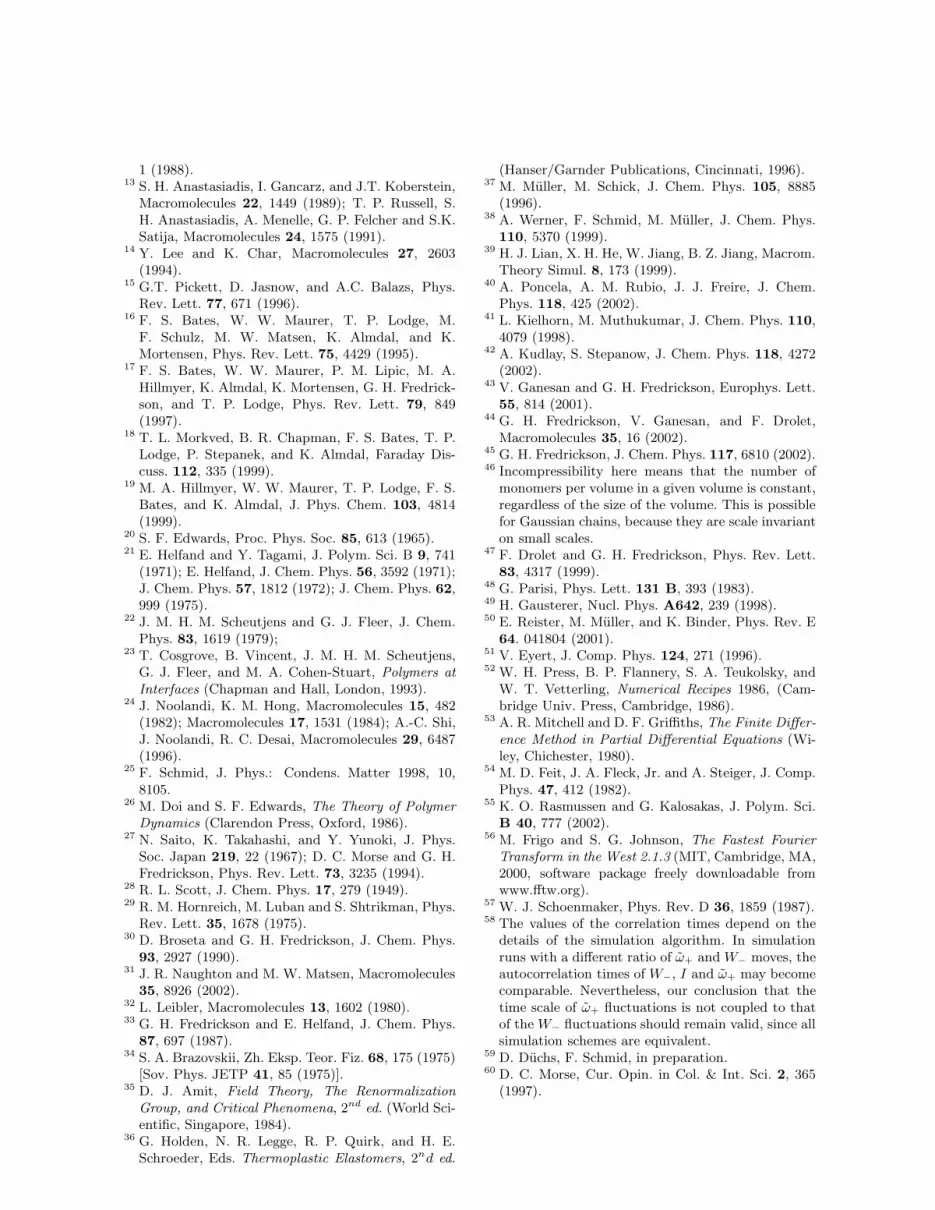
FIG. 17. Curvature radius DC (circles) and prefer-ential length scale, L0, as obtained from the maximumof S0(q) (squares) at χN = 12.5 in simulations on a48 × 48 lattice. Filled and empty symbols correspondto disordered and lamellar initial conditions, respec-tively. Dashed lines are guides for the eye.
To understand better what happens at the onsetof the microemulsion phase, we have calculated themean curvature diameter, DC , of the boundariesof A and B microdomains:
DC = 2
[
1
Lc
∫
ds
∣
∣
∣
∣
dt
ds
∣
∣
∣
∣
2]−1/2
, (44)
where Lc is the sum of all contour lengths of the mi-crodomain boundaries, and t is the tangent vectorat a given coordinate s along the contour. Detailsof the calculation of this object will be presentedelsewhere59. Furthermore, we examine the maxi-mum, qmax, of F0(q), which indicates the preferen-tial Fourier wave number of a configuration multi-plied by 2π. In turn, L/qmax =: L0 indicates the
preferential length scale of a configuration. Fig.17 compares DC and L0 for various homopoly-mer concentrations φH at χN = 12.5, for both L-started and D-started runs. Whereas for lower φH ,DC is larger than L0, the two lengths cross eachother as φH is increased. Thus we have identifiedthe mechanism by which fluctuations generate themicroemulsion phase: it forms when the width ofthe lamellae grows larger than the curvature radiusof the fluctuating boundaries, causing the lamellaeto break up. This type of “Lindemann criterion”for production of a bicontinuous microemulsion bymelting of a lamellar phase has discussed elsewherein the context of oil/water/surfactant phases60.
V. SUMMARY AND CONCLUSIONS
In the present paper, we have introduced a newway of evaluating the full partition function of asystem of polymeric blends subject to thermal fluc-tuations. The complex Langevin approach whichwas employed in our earlier researches, accountsfor both the W− and W+ fluctuations, and is ableto predict the shift in the order-disorder transi-tion at low φH and in the two-phase region. For0.7 <∼ φH <∼ 0.9 it runs into numerical difficul-ties. We believe that the large system sizes neces-sitated in such regions as well as the concomitantstrong fluctuation effects arising near the Lifshitzpoints restricts the applicability of the complexLangevin method in such regimes. As an alter-native, we have proposed a field-theoretic MonteCarlo approach, which was shown to be applicableto greater regions of the phase diagram. Small lat-tices (32×32) sufficed up to φH = 0.7, above whichbigger (48× 48) lattices had to be used. In the re-gion where both methods work, they are in goodagreement, indicating that theW+ fluctuations ne-glected in the latter simulations contribute only aminor correction. Further evidence for this circum-stance was found in empirical test runs. Such ob-servations also suggest that one could have poten-tially employed a real Langevin scheme where theW+ fluctuations are neglected50. Regretfully, how-ever, a full analysis of the W+ fluctuations was ren-dered difficult by the occurrence of a non-positive-definite weighting factor (the sign problem). Afluctuation-corrected phase diagram was presentedfor C=50, which corresponds well in qualitativeterms to the PEE/PDMS/PEE-PDMS system ofintermediate polymerization indices examined ina series of recent experiments16–19, providing fur-ther corroboration of the existence of a region ofbicontinuous microemulsion between the lamellarand phase-separated regions. The mechanism re-sponsible for the formation of this phase was shown
14
to be intimately related to matching length scalesof the curvature of microdomain boundaries andof the lamellar periodicity. In an upcoming arti-cle, we will examine properties of the disorderedphase59.
We have benefited from fruitful discussions withM. Schick, R. Netz, M. Matsen, and S. Sides. Thiswork was supported by the Deutsche Forschungs-gemeinschaft (Germany). VG and GHF were par-tially supported by the National Science Founda-tion under Awards DMR-02-04199 and DMR-98-70785, and the Petroleum Research Fund, admin-istered by the ACS. The Monte Carlo simulationswere carried out on the CRAY T3E of the NICinstitute in Julich.
APPENDIX: COMPLEX LANGEVIN
METHOD
In this appendix, we provide a brief outline ofthe complex Langevin method. Readers interestedin more details are referred to Ref.44. The com-plex Langevin technique involves generating W−
and W+ states in the entire complex plane (de-spite the fact that the integrations in Eq. (8) arerestricted to the real axis in W− and the imaginaryaxis in W+) by means of complex Langevin equa-tions. Specifically, the equations used to generatethe real and imaginary parts of the W− and W+
fields, WR− ,W
I−,W
R+ , and W I
+, are of the form:
∂[WR− (r, t) + iW I
−(r, t)]
∂t= −δH [W−,W+]
δW−(r, t)
+ θ(r, t), (45)
∂[W I+(r, t) − iWR
+ (r, t)]
∂t= −i δH [W−,W+]
δW+(r, t)
+θ(r, t), (46)
where θ(r, t) is a real Gaussian white noise withmoments satisfying the appropriate fluctuation-dissipation relation: 〈θ〉 = 0, 〈θ(r, t)θ(r′, t′)〉 =2δ(t− t′)δ(r − r′). In the above equations,
δH [W−,W+]
δW−(r)= C
[
2W−
χN− φA(r;W−,W+)
+ φB(r;W−,W+)
]
(47)
δH [W−,W+]
δW+(r)= C [φA(r;W−,W+)
+ φB(r;W−,W+) − 1] (48)
The evolution of the WR− ,W
I− and WR
+ ,WI+ fields
according to the above Langevin equations (45 -
46) produces in the long-time limit the generationof field states such that the “time” averages ac-quire the same values as those computed using theoriginal non-positive-definite Boltzmann weight48.Equilibration of the simulation can be establishedby monitoring an appropriate quantity, such asthe average of the imaginary component of en-ergy/densities which should identically vanish atequilibrium. We note that with such an averagingprocedure, physical observables such as the aver-age A monomer density, φA = 〈φA〉, turn out tobe real, while their fluctuating analogs such as φAare generally complex.
It is pertinent to note a few special features ofthe complex Langevin equations (45 - 46). In theabsence of the noise term θ(r, t), the dynamics willdrive the system to the nearest saddle point. Con-sequently, it is straightforward to probe the sta-bility of the mean-field solutions within the CLsimulation scheme by setting the noise term identi-cally to zero. Furthermore, this feature enables thesampling in the presence of the noise to be auto-matically confined near a saddle point, avoiding along equilibration period if the system were to beprepared in an initial configuration far from thesaddle point.
1 D.R. Paul and S. Newman, Polymer Blends (Aca-demic Press, New York, 1978).
2 K. Solc (edt.), Polymer Compatibility and Incompat-
ibility (Harwood Academic Publishers, Chur, 1980).3 P. Flory, Principles of Polymer Chemistry (CornellUniversity Press, Ithaca, New York, 1971).
4 K. Binder, Adv. Polymer Sci.112, 181 (1994).5 P. G. de Gennes, Scaling Concepts in Polymer
Physics (Cornell University Press, Ithaca, NewYork, 1979).
6 J. H. Hildebrand, R. L. Scott, The solubility of non-
electrolytes Dover, New York, (1964).7 F.S. Bates and G.H. Fredrickson, Annu. Rev. Phys.Chem. 41, 25 (1990); F.S. Bates, Science 251, 898(1991).
8 R. Israels et al, J. Chem. Phys. 102, 8149 (1995).9 R. Holyst and M. Schick, J. Chem. Phys. 96, 7728(1992).
10 M. W. Matsen and M. Schick, Phys. Rev. Lett. 72,2660 (1994); M.W. Matsen, Phys. Rev. Lett. 74,4225 (1995); Macromolecules 28, 5765 (1995); J.Physics: Cond. Matt. 14, R21 (2001).
11 H. S. Jeon, J. H. Lee, and N. P. Balsara,Phys.Rev.Lett. 79, 3275 (1997); Macromolecules31, 3328 (1998); Macromolecules 31, 3340 (1998).
12 L. Leibler, Makromol. Chem., Macromol. Symp. 16,
15
1 (1988).13 S. H. Anastasiadis, I. Gancarz, and J.T. Koberstein,
Macromolecules 22, 1449 (1989); T. P. Russell, S.H. Anastasiadis, A. Menelle, G. P. Felcher and S.K.Satija, Macromolecules 24, 1575 (1991).
14 Y. Lee and K. Char, Macromolecules 27, 2603(1994).
15 G.T. Pickett, D. Jasnow, and A.C. Balazs, Phys.Rev. Lett. 77, 671 (1996).
16 F. S. Bates, W. W. Maurer, T. P. Lodge, M.F. Schulz, M. W. Matsen, K. Almdal, and K.Mortensen, Phys. Rev. Lett. 75, 4429 (1995).
17 F. S. Bates, W. W. Maurer, P. M. Lipic, M. A.Hillmyer, K. Almdal, K. Mortensen, G. H. Fredrick-son, and T. P. Lodge, Phys. Rev. Lett. 79, 849(1997).
18 T. L. Morkved, B. R. Chapman, F. S. Bates, T. P.Lodge, P. Stepanek, and K. Almdal, Faraday Dis-cuss. 112, 335 (1999).
19 M. A. Hillmyer, W. W. Maurer, T. P. Lodge, F. S.Bates, and K. Almdal, J. Phys. Chem. 103, 4814(1999).
20 S. F. Edwards, Proc. Phys. Soc. 85, 613 (1965).21 E. Helfand and Y. Tagami, J. Polym. Sci. B 9, 741
(1971); E. Helfand, J. Chem. Phys. 56, 3592 (1971);J. Chem. Phys. 57, 1812 (1972); J. Chem. Phys. 62,999 (1975).
22 J. M. H. M. Scheutjens and G. J. Fleer, J. Chem.Phys. 83, 1619 (1979);
23 T. Cosgrove, B. Vincent, J. M. H. M. Scheutjens,G. J. Fleer, and M. A. Cohen-Stuart, Polymers at
Interfaces (Chapman and Hall, London, 1993).24 J. Noolandi, K. M. Hong, Macromolecules 15, 482
(1982); Macromolecules 17, 1531 (1984); A.-C. Shi,J. Noolandi, R. C. Desai, Macromolecules 29, 6487(1996).
25 F. Schmid, J. Phys.: Condens. Matter 1998, 10,8105.
26 M. Doi and S. F. Edwards, The Theory of Polymer
Dynamics (Clarendon Press, Oxford, 1986).27 N. Saito, K. Takahashi, and Y. Yunoki, J. Phys.
Soc. Japan 219, 22 (1967); D. C. Morse and G. H.Fredrickson, Phys. Rev. Lett. 73, 3235 (1994).
28 R. L. Scott, J. Chem. Phys. 17, 279 (1949).29 R. M. Hornreich, M. Luban and S. Shtrikman, Phys.
Rev. Lett. 35, 1678 (1975).30 D. Broseta and G. H. Fredrickson, J. Chem. Phys.
93, 2927 (1990).31 J. R. Naughton and M. W. Matsen, Macromolecules
35, 8926 (2002).32 L. Leibler, Macromolecules 13, 1602 (1980).33 G. H. Fredrickson and E. Helfand, J. Chem. Phys.
87, 697 (1987).34 S. A. Brazovskii, Zh. Eksp. Teor. Fiz. 68, 175 (1975)
[Sov. Phys. JETP 41, 85 (1975)].35 D. J. Amit, Field Theory, The Renormalization
Group, and Critical Phenomena, 2nd ed. (World Sci-entific, Singapore, 1984).
36 G. Holden, N. R. Legge, R. P. Quirk, and H. E.Schroeder, Eds. Thermoplastic Elastomers, 2nd ed.
(Hanser/Garnder Publications, Cincinnati, 1996).37 M. Muller, M. Schick, J. Chem. Phys. 105, 8885
(1996).38 A. Werner, F. Schmid, M. Muller, J. Chem. Phys.
110, 5370 (1999).39 H. J. Lian, X. H. He, W. Jiang, B. Z. Jiang, Macrom.
Theory Simul. 8, 173 (1999).40 A. Poncela, A. M. Rubio, J. J. Freire, J. Chem.
Phys. 118, 425 (2002).41 L. Kielhorn, M. Muthukumar, J. Chem. Phys. 110,
4079 (1998).42 A. Kudlay, S. Stepanow, J. Chem. Phys. 118, 4272
(2002).43 V. Ganesan and G. H. Fredrickson, Europhys. Lett.
55, 814 (2001).44 G. H. Fredrickson, V. Ganesan, and F. Drolet,
Macromolecules 35, 16 (2002).45 G. H. Fredrickson, J. Chem. Phys. 117, 6810 (2002).46 Incompressibility here means that the number of
monomers per volume in a given volume is constant,regardless of the size of the volume. This is possiblefor Gaussian chains, because they are scale invarianton small scales.
47 F. Drolet and G. H. Fredrickson, Phys. Rev. Lett.83, 4317 (1999).
48 G. Parisi, Phys. Lett. 131 B, 393 (1983).49 H. Gausterer, Nucl. Phys. A642, 239 (1998).50 E. Reister, M. Muller, and K. Binder, Phys. Rev. E
64. 041804 (2001).51 V. Eyert, J. Comp. Phys. 124, 271 (1996).52 W. H. Press, B. P. Flannery, S. A. Teukolsky, and
W. T. Vetterling, Numerical Recipes 1986, (Cam-bridge Univ. Press, Cambridge, 1986).
53 A. R. Mitchell and D. F. Griffiths, The Finite Differ-
ence Method in Partial Differential Equations (Wi-ley, Chichester, 1980).
54 M. D. Feit, J. A. Fleck, Jr. and A. Steiger, J. Comp.Phys. 47, 412 (1982).
55 K. O. Rasmussen and G. Kalosakas, J. Polym. Sci.B 40, 777 (2002).
56 M. Frigo and S. G. Johnson, The Fastest Fourier
Transform in the West 2.1.3 (MIT, Cambridge, MA,2000, software package freely downloadable fromwww.fftw.org).
57 W. J. Schoenmaker, Phys. Rev. D 36, 1859 (1987).58 The values of the correlation times depend on the
details of the simulation algorithm. In simulationruns with a different ratio of ω+ and W− moves, theautocorrelation times of W−, I and ω+ may becomecomparable. Nevertheless, our conclusion that thetime scale of ω+ fluctuations is not coupled to thatof the W− fluctuations should remain valid, since allsimulation schemes are equivalent.
59 D. Duchs, F. Schmid, in preparation.60 D. C. Morse, Cur. Opin. in Col. & Int. Sci. 2, 365