Journal of Loss Prevention in the Process Industries 11 (1998) 135–148

Design of a computer tool for the evaluation of the consequencesof accidental natural gas releases in distribution pipes

J. Arnaldos, J. Casal*, H. Montiel, M. Sanchez-Carricondo, J.A. Vı´lchezCentre d’Estudis del Risc Tecnolo`gic (CERTEC). Department of Chemical Engineering, Universitat Polite`cnica de Catalunya-Institut d’Estudis

Catalans Diagonal 647. 08028-Barcelona, Catalonia, Spain

Accepted 20 November 1997

Abstract

A computer system was designed to model releases of a gas to the atmosphere. This paper describes the mathematical modelsused to describe the phenomenon: source term (which can be applied to gases with an ideal behaviour), turbulent jet, jet fire(including thermal radiation vulnerability models) and atmospheric dispersion (both for light and neutral gases), as well as thesoftware and hardware used in the system. 1997 Elsevier Science Ltd. All rights reserved.

Keywords:Risk analysis; Major accidents; Loss prevention

Nomenclature

A9 parameter in Eq. (11)

FA9 =m0sub

(k21)Qm0sub

(12B)1/2G, -

Ac area of the cross section of the pipe, m2

Aor hole area, m2

b characteristic plume width, m

parameter in Eq. (11)FB = S Pa

P0subD(k21)/kG, -B

C gas concentration, mol fractionCLOC level of concern for isopleth definition, mol

fraction

parameter in Eq. (11)FC9 =22kk21G, -C9

D pipe diameter, m or mmDor hole diameter, mmEp emissive power of fire, kW/m2

F view factor, -F(t) function in Eq. (6) and Eq. (7)

FF(t) =1

1 + aso·tG, -

f friction factor, -

* Corresponding author.

0950–4230 /98 /$19.00 1997 Elsevier Science Ltd. All rights reserved.PII: S0950-4230 (97)00041-7

G mass flux, kg/m2sh height of the release point, mk heat capacity ratio, -K pressure drop coefficient for each fitting, -L pipe length, mLe equivalent pipe length, mLF flame length, mm mass of gas contained in the pipe, kgM molecular weight, kg/kmolMa Mach number (u/uso), -P pressure, Pa or bar absPa atmospheric pressure, Pa or bar absPW vapour pressure of water in the atmosphere, Paqr incident thermal radiation per unit surface,

kW/m2

Qm mass discharge rate, kg/s or Nm3/hQmax maximum flow-rate, kg/s or Nm3/hR ideal gas constant, J/kmol·KRe Reynolds number (Dur/m), -S flame displacement, mT temperature, Kt time, su velocity of the gas, m/suso velocity of the sound (for ideal gases uso =

(k·M/(R·T))1/2), m/suW wind velocity, m/sx horizontal co-ordinate or distance, my co-ordinate or width, m

136 J. Arnaldos et al. / Journal of Loss Prevention in the Process Industries 11 (1998) 135–148

parameter in Eq. (4)FY = 1 + Sk212 D·Ma2G, -Y

z vertical co-ordinate or distance, m

Greek letters

a flame tilt, °

aso parameter in F(t)Faso =Qm0·(k21)

2·m0G, s21

F parameter in Eq. (11)FF =T(t)T0sub

G, -

l turbulent Schmidt number (constant value,equal to 1.16), -

m gas viscosity, kg/m·su angle between plume axis and horizontal (0 to

p/2 or 0 to2p/2), radiansr gas density, kg/m3

sy atmospheric dispersion coefficient in the ydirection, m

sz atmospheric dispersion coefficient in the zdirection, m

t atmospheric transmissivity, -

Subscripts

b bottom plume isopletht top plume isopleth0 steady-state0sub steady state or initial values in subsonic flow1 at the beginning of the pipe2 inside the pipe and on a level with the hole* plume centreline

1. Introduction

Natural gas is one of the most widely used domesticfuels in industrialized countries, and its consumption iscontinuously increasing. As a result, complex piping sys-tems have been installed – and are being enlarged – totransport and distribute the gas, both for electricity gen-eration and as a domestic fuel. These piping networksare mostly installed in urban zones, i.e. in highly popu-lated areas. Therefore, accidental gas releases can causesignificant economic losses as well as injury to the popu-lation.

Although gas piping systems are mostly installedunderground, they are often damaged by various activi-ties. A recent historical analysis of 185 accidents(Montiel et al., 1996) has shown that approximately 67%of accidents involving natural gas occur in piping sys-tems. The most frequent causes were mechanical failure,impact failure, human error and external events.Amongst impact failure accidents (39) the most frequent

cause was excavating machinery (21), followed byvehicles (5) and heavy objects (5).

These accidents may result in the perforation of thepipe or even in its complete fracture. Gas will bereleased to the environment at a flow-rate depending onthe hole diameter and the pressure in the pipe until therelease is stopped automatically by means of a regulator(reaction to excessive flow-rate) or by hand; the releaseflow-rate will then decrease until the end of the emerg-ency.

A computer code allowing rapid real-time estimationof the potential effects of gas release would be very use-ful in managing such an accident: gas dispersion couldbe simulated, safety distances could be established fromthe knowledge of the gas concentrations in the atmos-phere near the release point, the thermal radiation causedby a jet fire could also be estimated, and the amount ofgas released could be determined. These calculationscould also predict the consequences of any hypotheticalsituation, in order to assess new installations or just toanalyse the risk of a given gas distribution system.

This computer code should cover everything from thecalculation of the flow-rate at which gas is released, upto the ultimate consequences of the release (for example,the number of people injured or killed by thermal radi-ation in the case of ignition). It should be usable by non-experts; this means that it should accept, in addition tothe very comprehensive information available for predic-tive situations, the rather simple descriptions of accidentsusually available in fast real-time use.

This communication presents such a system. A set ofmathematical models were implemented by computer, inaccordance with the previous conditions, to allow thecalculation of gas flow-rate, gas dispersion and thermalradiation from a fire jet. A user-friendly environmentwas designed, in order to obtain a simple but usefulinteractive system.

2. Mathematical models

A set of mathematical models were implemented,covering the following aspects:

1. source term2. turbulent gas jet3. jet fire4. atmospheric gas dispersion, with two cases:1. integral plume2. neutral gas dispersion.

In the following paragraphs these models are brieflymentioned.

2.1. Source term

To study the release of a gas, the existing modelsdescribe two situations:

137J. Arnaldos et al. / Journal of Loss Prevention in the Process Industries 11 (1998) 135–148

a) ‘Hole models’, in which the gas flows through ahole in the wall of a tank. Unsteady state is not takeninto account (as the pressure inside the tank is consideredto be constant) and the model does not take into accountany changes in gas exit velocity or in pressure drop inthe pipe. This model can be applied to the release of agas from a pipe if the hole is small; however, for largeholes the model overpredicts the flow-rate.

b) ‘Pipe models’, in which gas flows through a holewhich corresponds to the complete breaking of the pipe.Adiabatic flow and isentropic release are assumed; aconstant pressure is also assumed at an initial point inthe pipe, and pressure drop along it is taken into account.This model gives good predictions for complete fractureof the pipe, but it cannot be applied to flow through holeswith a diameter smaller than the pipe diameter.

These two models cannot be applied, therefore, to allthe cases ranging from a relatively small hole up to alarge one with a diameter smaller than that of the pipe.Furthermore, they do not take into account the unsteady-state flow found when a safety device is closed and theflow-rate decreases progressively.

Therefore, a new model bridging this gap wasdeveloped. The following hypotheses were assumed:flow essentially 1D, ideal gas properties, adiabatic flowin the pipe and isentropic flow at the release point. Then,by applying the energy and momentum equations, thefollowing equation was obtained:

k + 1k

lnSP1T2

P2T1D +

MRG2 SP2

2

T22

P21

T1D + S4fLe

D D = 0 (1)

Based on this equation, the model was developed forthe different possible situations which can be found insteady state:

1. subsonic flow in the pipe, sonic flow at the hole2. subsonic flow in the pipe and at the hole3. sonic flow in the pipe (at a point level with the hole)

and at the hole.

The model was also applied to unsteady state, i.e. thesituation found if, some time after the beginning of therelease, the gas feed into the system is stopped; fromthat moment on, the release flow-rate will decrease untilthe end of the emergency. A fourth-order Runge-Kuttamethod was used to solve the set of equations numeri-cally.

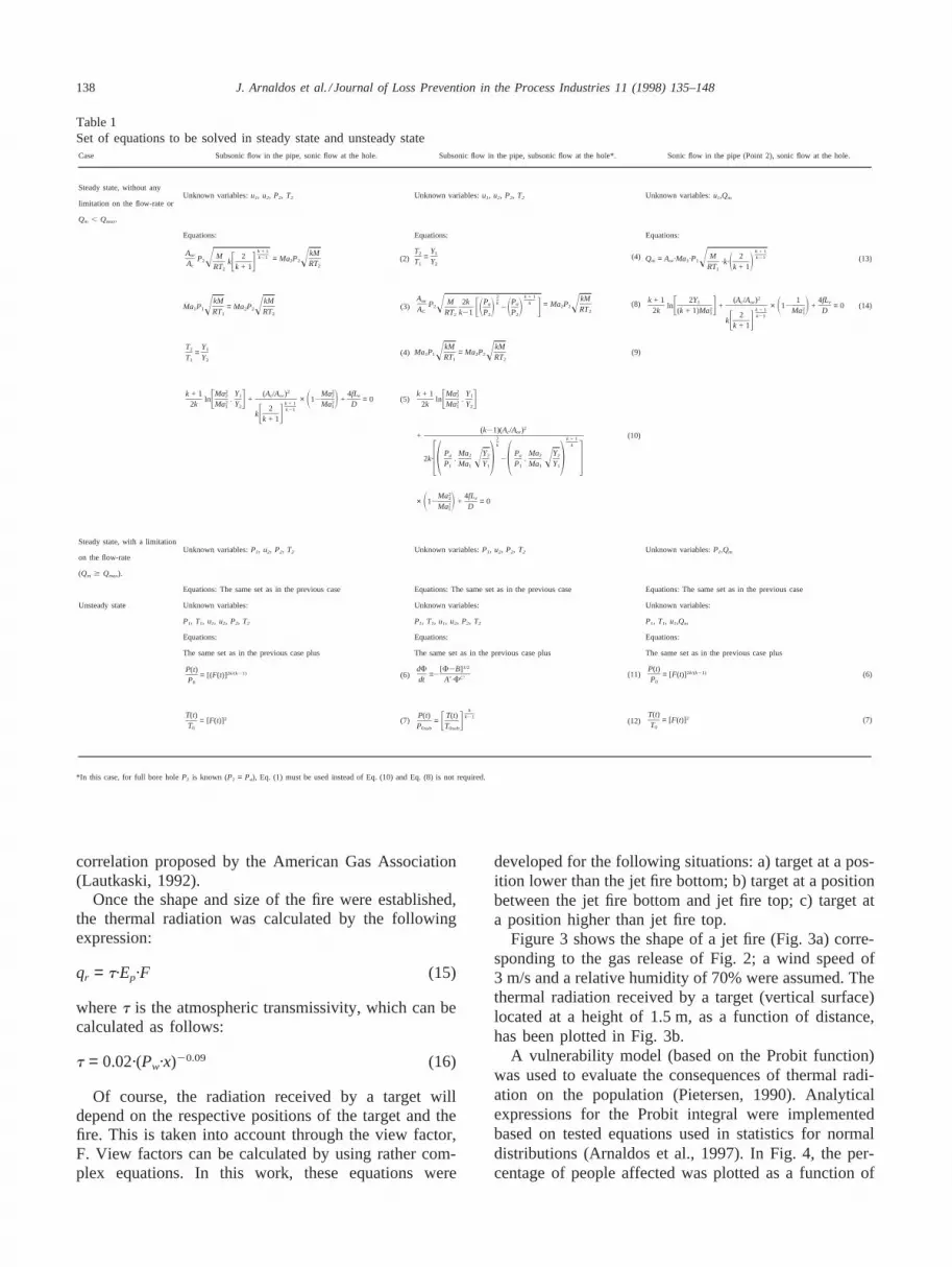
Table 1 shows the sets of equations to be solved foreach case in steady state and unsteady state.

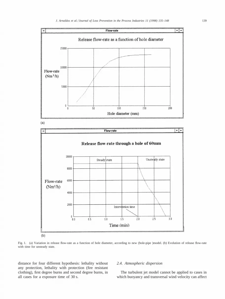
Figure 1a shows the variation in the release flow-rateas a function of hole diameter for a given case (releaseof natural gas; pipe length, 1000 m; pressure, 5 bar abs;temperature, 20°C; pipe i.d., 163.6 mm; fittings, 13 T’sof 90° (K = 0.5)), as predicted by the model in steady

state. Fig. 1b shows the variation in the release flow-rateas a function of time, for the aforementioned case butconsidering only a hole diameter of 60 mm, as predictedby the model in unsteady state. This new model has beendescribed in detail elsewhere (Montiel et al., submitted).

2.2. Turbulent gas jet

When a gas is released through a hole at high speed,it is dispersed in the atmosphere as a jet which can beassumed to be conical. The field of velocities in this jetis much higher than that of the wind; this implies a highdegree of turbulence, which causes the entrainment ofair and a more intense dispersion than in a release takingplace with an initial velocity that is practically equal tozero. In the jet, the velocity profile varies from a top-hat velocity profile at the beginning to a Gaussian profileonce the jet is fully developed (with the maximum valueat the jet axis). A fully developed turbulent jet is charac-terized by a value of the Reynolds number Re. 2.5 ×104 (TNO, 1992).

The model selected for the present work can beapplied to turbulent jets, free (i.e. without any obstacleswhich could hinder their expansion) and without sig-nificant wind speed (uw , 1 m/s). It is assumed that thejet is fully developed. The model was based on the equa-tions proposed by TNO (1992).

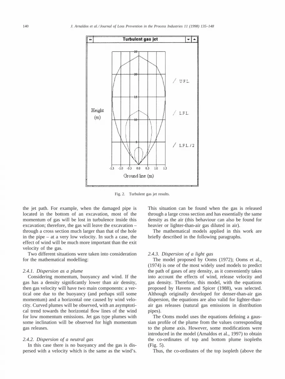
Figure 2 shows the prediction of the jet profile for thesame case as in the previous section, considering only ahole diameter of 60 mm. The shape of a vertical turbu-lent jet was plotted for three concentrations: the U. F.L. (15% in volume for natural gas), the L. F. L. (5% invol.) and 50% of the L. F. L. (2.5% in vol.), which couldbe considered as a ‘safety value’. As can be observed,the jet would have a length of 24 m for the 2.5% vol.concentration, with a diameter of approximately 1.5 m.

2.3. Jet fire

If the gas released through a damaged pipe meets anignition source, a jet fire will occur. The shape and sizeof the fire must be known to calculate its thermal radi-ation. Two cases must be taken into account: no wind,and a significant wind speed.

For the cases in which there is no wind, the modelproposed by Hawthorne et al. (1949) was taken. Thispredicts the length of the jet fire, the distance from therelease point at which the flame initiates and themaximum diameter of the flame.

For those cases in which there is a significant windspeed, the model proposed by Kalghatgi (1983) wasused. This author considered the jet fire to be a frustumof a cone, with a certain inclination with respect to thevertical caused by the wind. Kalghatgi’s model allowsthe calculation of the dimensions of the fire. Flame tiltas a function of wind velocity can be calculated with the

138 J. Arnaldos et al. / Journal of Loss Prevention in the Process Industries 11 (1998) 135–148

Table 1Set of equations to be solved in steady state and unsteady stateCase Subsonic flow in the pipe, sonic flow at the hole. Subsonic flow in the pipe, subsonic flow at the hole*. Sonic flow in the pipe (Point 2), sonic flow at the hole.

Steady state, without anyUnknown variables:u1, u2, P2, T2 Unknown variables:u1, u2, P2, T2 Unknown variables:u1,Qm

limitation on the flow-rate or

Qm , Qmax.

Equations: Equations: Equations:

T2

T1=

Y1

Y2(4)Aor

AcP2! M

RT2

kF 2k + 1G

k + 1k21 = Ma2P2!kM

RT2(2) Qm = Aor·Ma1·P1! M

RT1

·k·S 2k + 1D

k + 1k21 (13)

Aor

ACP2! M

RT2

2kk21 FSPa

P2D 2

k2SPa

P2D k + 1

k G = Ma2P2!kMRT2

(8) k + 12k

lnF 2Y1

(k + 1)Ma21G +

(Ac/Aor)2

kF 2k + 1G

k + 1k21

× S121

Ma21D +

4fLe

D= 0 (14)Ma1P1!kM

RT1= Ma2P2!kM

RT2(3)

Ma1P1!kMRT1

= Ma2P2!kMRT2

(9)T2

T1

=Y1

Y2

(4)

k + 12k

lnFMa22

Ma21

.Y1

Y2G +

(Ac/Aor)2

kF 2k + 1G

k + 1k21

× S12Ma2

2

Ma21D +

4fLe

D= 0 (5)

k + 12k

lnFMa22

Ma21

.Y1

Y2G

+(k21)(Ac/Aor)2

2k·31 Pa

P1.Ma2

Ma1!Y2

Y122k

21 Pa

P1.Ma2

Ma1!Y2

Y12k + 1

k

4(10)

× S12Ma2

2

Ma21D +

4fLe

D= 0

Steady state, with a limitationUnknown variables:P1, u2, P2, T2 Unknown variables:P1, u2, P2, T2 Unknown variables:P1,Qm

on the flow-rate

(Qm $ Qmax).

Equations: The same set as in the previous case Equations: The same set as in the previous case Equations: The same set as in the previous case

Unsteady state Unknown variables: Unknown variables: Unknown variables:

P1, T1, u1, u2, P2, T2 P1, T1, u1, u2, P2, T2 P1, T1, u1,Qm

Equations: Equations: Equations:

The same set as in the previous case plus The same set as in the previous case plus The same set as in the previous case plus

dF

dt=2

[F2B]1/2

A9·FC9(11)

P(t)P0

= [F(t)]2k/(k21) (6)P(t)P0

= [(F(t)]2k/(k21) (6)

T(t)T0

= [F(t)]2 (7)T(t)T0

= [F(t)]2 (7)P(t)P0sub

= FT(t)T0sub

G k

k21(12)

*In this case, for full bore holeP2 is known (P2 = Pa), Eq. (1) must be used instead of Eq. (10) and Eq. (8) is not required.

correlation proposed by the American Gas Association(Lautkaski, 1992).

Once the shape and size of the fire were established,the thermal radiation was calculated by the followingexpression:

qr = t·Ep·F (15)

wheret is the atmospheric transmissivity, which can becalculated as follows:

t = 0.02·(Pw·x)20.09 (16)

Of course, the radiation received by a target willdepend on the respective positions of the target and thefire. This is taken into account through the view factor,F. View factors can be calculated by using rather com-plex equations. In this work, these equations were

developed for the following situations: a) target at a pos-ition lower than the jet fire bottom; b) target at a positionbetween the jet fire bottom and jet fire top; c) target ata position higher than jet fire top.

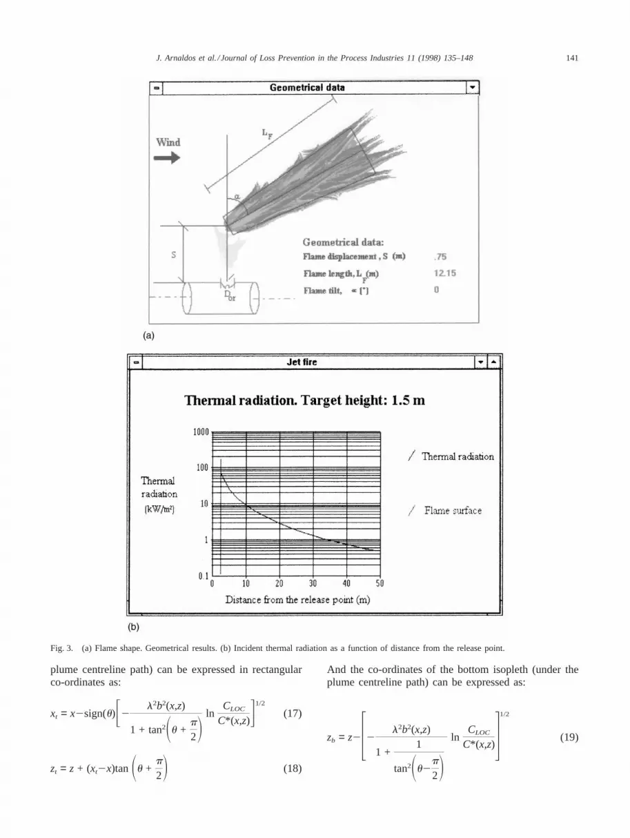
Figure 3 shows the shape of a jet fire (Fig. 3a) corre-sponding to the gas release of Fig. 2; a wind speed of3 m/s and a relative humidity of 70% were assumed. Thethermal radiation received by a target (vertical surface)located at a height of 1.5 m, as a function of distance,has been plotted in Fig. 3b.

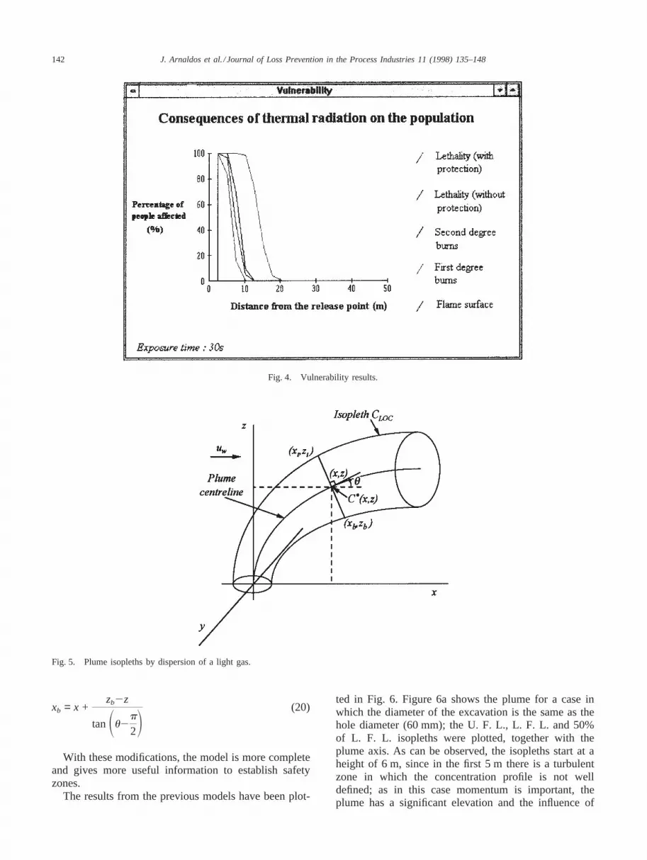
A vulnerability model (based on the Probit function)was used to evaluate the consequences of thermal radi-ation on the population (Pietersen, 1990). Analyticalexpressions for the Probit integral were implementedbased on tested equations used in statistics for normaldistributions (Arnaldos et al., 1997). In Fig. 4, the per-centage of people affected was plotted as a function of

139J. Arnaldos et al. / Journal of Loss Prevention in the Process Industries 11 (1998) 135–148

Fig. 1. (a) Variation in release flow-rate as a function of hole diameter, according to new (hole-pipe )model. (b) Evolution of release flow-ratewith time for unsteady state.

distance for four different hypothesis: lethality withoutany protection, lethality with protection (fire resistantclothing), first degree burns and second degree burns, inall cases for a exposure time of 30 s.

2.4. Atmospheric dispersion

The turbulent jet model cannot be applied to cases inwhich buoyancy and transversal wind velocity can affect

140 J. Arnaldos et al. / Journal of Loss Prevention in the Process Industries 11 (1998) 135–148

Fig. 2. Turbulent gas jet results.

the jet path. For example, when the damaged pipe islocated in the bottom of an excavation, most of themomentum of gas will be lost in turbulence inside thisexcavation; therefore, the gas will leave the excavation –through a cross section much larger than that of the holein the pipe – at a very low velocity. In such a case, theeffect of wind will be much more important than the exitvelocity of the gas.

Two different situations were taken into considerationfor the mathematical modelling:

2.4.1. Dispersion as a plumeConsidering momentum, buoyancy and wind. If the

gas has a density significantly lower than air density,then gas velocity will have two main components: a ver-tical one due to the buoyancy (and perhaps still somemomentum) and a horizontal one caused by wind velo-city. Curved plumes will be observed, with an asymptoti-cal trend towards the horizontal flow lines of the windfor low momentum emissions. Jet gas type plumes withsome inclination will be observed for high momentumgas releases.

2.4.2. Dispersion of a neutral gasIn this case there is no buoyancy and the gas is dis-

persed with a velocity which is the same as the wind’s.

This situation can be found when the gas is releasedthrough a large cross section and has essentially the samedensity as the air (this behaviour can also be found forheavier or lighter-than-air gas diluted in air).

The mathematical models applied in this work arebriefly described in the following paragraphs.

2.4.3. Dispersion of a light gasThe model proposed by Ooms (1972); Ooms et al.,

(1974) is one of the most widely used models to predictthe path of gases of any density, as it conveniently takesinto account the effects of wind, release velocity andgas density. Therefore, this model, with the equationsproposed by Havens and Spicer (1988), was selected.Although originally developed for denser-than-air gasdispersion, the equations are also valid for lighter-than-air gas releases (natural gas emissions in distributionpipes).

The Ooms model uses the equations defining a gaus-sian profile of the plume from the values correspondingto the plume axis. However, some modifications wereintroduced in the model (Arnaldos et al., 1997) to obtainthe co-ordinates of top and bottom plume isopleths(Fig. 5).

Thus, the co-ordinates of the top isopleth (above the

141J. Arnaldos et al. / Journal of Loss Prevention in the Process Industries 11 (1998) 135–148

Fig. 3. (a) Flame shape. Geometrical results. (b) Incident thermal radiation as a function of distance from the release point.

plume centreline path) can be expressed in rectangularco-ordinates as:

xt = x2sign(u)F2l2b2(x,z)

1 + tan2Su +p

2Dln

CLOC

C*(x,z)G1/2

(17)

zt = z + (xt2x)tanSu +p

2D (18)

And the co-ordinates of the bottom isopleth (under theplume centreline path) can be expressed as:

zb = z232l2b2(x,z)

1 +1

tan2Su2p

2Dln

CLOC

C*(x,z)41/2

(19)

142 J. Arnaldos et al. / Journal of Loss Prevention in the Process Industries 11 (1998) 135–148

Fig. 4. Vulnerability results.

Fig. 5. Plume isopleths by dispersion of a light gas.

xb = x +zb2z

tanSu2p

2D(20)

With these modifications, the model is more completeand gives more useful information to establish safetyzones.

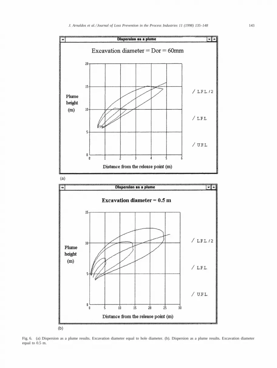
The results from the previous models have been plot-

ted in Fig. 6. Figure 6a shows the plume for a case inwhich the diameter of the excavation is the same as thehole diameter (60 mm); the U. F. L., L. F. L. and 50%of L. F. L. isopleths were plotted, together with theplume axis. As can be observed, the isopleths start at aheight of 6 m, since in the first 5 m there is a turbulentzone in which the concentration profile is not welldefined; as in this case momentum is important, theplume has a significant elevation and the influence of

143J. Arnaldos et al. / Journal of Loss Prevention in the Process Industries 11 (1998) 135–148

Fig. 6. (a) Dispersion as a plume results. Excavation diameter equal to hole diameter. (b). Dispersion as a plume results. Excavation diameterequal to 0.5 m.

144 J. Arnaldos et al. / Journal of Loss Prevention in the Process Industries 11 (1998) 135–148

wind speed is relatively low. The results are similar tothose obtained with the turbulent gas jet describedabove.

In Fig. 6b the plume was plotted for the same case,but for an equivalent excavation diameter much largerthan the hole diameter (0.5 m). Now the gas has practi-cally no momentum; as a result, the elevation of theplume is only due to buoyancy, the turbulence zone isshorter and the influence of wind is much moreimportant. Considering the length of the plume path, theresults tend towards those obtained with the neutral gasdispersion model (the differences can be explained bybuoyancy and by the fact that the Ooms-model formu-lation is totally different from neutral gas dispersion).

2.4.4. Dispersion of a neutral gasThe well-known Pasquill-Gifford model was used

(Pasquill, 1962); according to this model, the concen-tration in a point of the plume can be calculated by thefollowing expression:

C(x,y,z) =Qm

2puwsysz

expS2y2

2s2yD* (21)

FexpS2(z2h)2

2s2zD + expS2

(z + h)2

2s2z

DGTo estimate the values of the atmospheric dispersion

coefficients, the model proposed by TNO (1992) wasused. The different equations of the model are notdescribed here, as they can be found in many environ-mental textbooks.

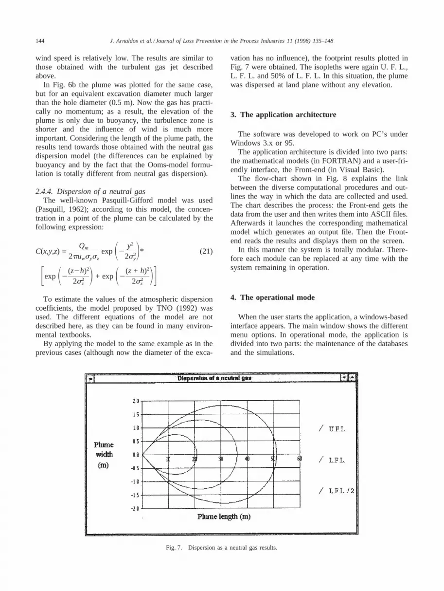
By applying the model to the same example as in theprevious cases (although now the diameter of the exca-

Fig. 7. Dispersion as a neutral gas results.

vation has no influence), the footprint results plotted inFig. 7 were obtained. The isopleths were again U. F. L.,L. F. L. and 50% of L. F. L. In this situation, the plumewas dispersed at land plane without any elevation.

3. The application architecture

The software was developed to work on PC’s underWindows 3.x or 95.

The application architecture is divided into two parts:the mathematical models (in FORTRAN) and a user-fri-endly interface, the Front-end (in Visual Basic).

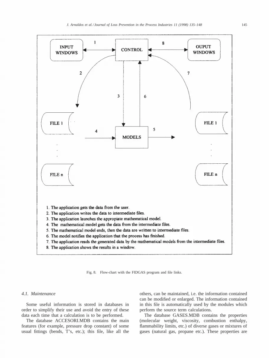
The flow-chart shown in Fig. 8 explains the linkbetween the diverse computational procedures and out-lines the way in which the data are collected and used.The chart describes the process: the Front-end gets thedata from the user and then writes them into ASCII files.Afterwards it launches the corresponding mathematicalmodel which generates an output file. Then the Front-end reads the results and displays them on the screen.

In this manner the system is totally modular. There-fore each module can be replaced at any time with thesystem remaining in operation.

4. The operational mode

When the user starts the application, a windows-basedinterface appears. The main window shows the differentmenu options. In operational mode, the application isdivided into two parts: the maintenance of the databasesand the simulations.

145J. Arnaldos et al. / Journal of Loss Prevention in the Process Industries 11 (1998) 135–148

Fig. 8. Flow-chart with the FIDGAS program and file links.

4.1. Maintenance

Some useful information is stored in databases inorder to simplify their use and avoid the entry of thesedata each time that a calculation is to be performed.

The database ACCESORI.MDB contains the mainfeatures (for example, pressure drop constant) of someusual fittings (bends, T’s, etc.); this file, like all the

others, can be maintained, i.e. the information containedcan be modified or enlarged. The information containedin this file is automatically used by the modules whichperform the source term calculations.

The database GASES.MDB contains the properties(molecular weight, viscosity, combustion enthalpy,flammability limits, etc.) of diverse gases or mixtures ofgases (natural gas, propane etc.). These properties are

146 J. Arnaldos et al. / Journal of Loss Prevention in the Process Industries 11 (1998) 135–148

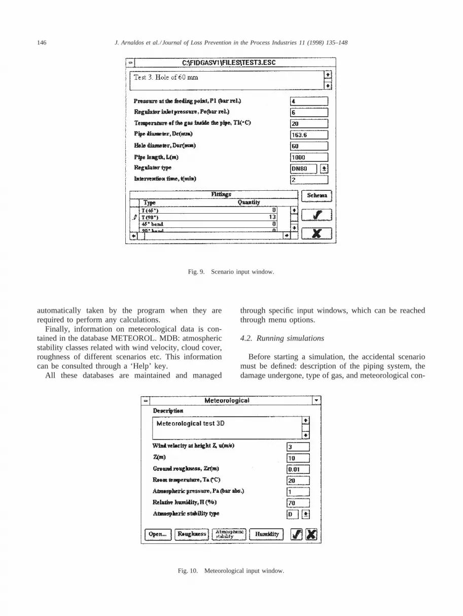
Fig. 9. Scenario input window.

automatically taken by the program when they arerequired to perform any calculations.

Finally, information on meteorological data is con-tained in the database METEOROL. MDB: atmosphericstability classes related with wind velocity, cloud cover,roughness of different scenarios etc. This informationcan be consulted through a ‘Help’ key.

All these databases are maintained and managed

Fig. 10. Meteorological input window.

through specific input windows, which can be reachedthrough menu options.

4.2. Running simulations

Before starting a simulation, the accidental scenariomust be defined: description of the piping system, thedamage undergone, type of gas, and meteorological con-

147J. Arnaldos et al. / Journal of Loss Prevention in the Process Industries 11 (1998) 135–148

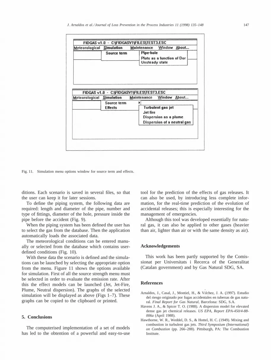
Fig. 11. Simulation menu options window for source term and effects.

ditions. Each scenario is saved in several files, so thatthe user can keep it for later sessions.

To define the piping system, the following data arerequired: length and diameter of the pipe, number andtype of fittings, diameter of the hole, pressure inside thepipe before the accident (Fig. 9).

When the piping system has been defined the user hasto select the gas from the database. Then the applicationautomatically loads the associated data.

The meteorological conditions can be entered manu-ally or selected from the database which contains user-defined conditions (Fig. 10).

With these data the scenario is defined and the simula-tions can be launched by selecting the appropriate optionfrom the menu. Figure 11 shows the options availablefor simulation. First of all the source strength menu mustbe selected in order to evaluate the emission rate. Afterthis the effect models can be launched (Jet, Jet-Fire,Plume, Neutral dispersion). The graphs of the selectedsimulation will be displayed as above (Figs 1–7). Thesegraphs can be copied to the clipboard or printed.

5. Conclusions

The computerised implementation of a set of modelshas led to the obtention of a powerful and easy-to-use

tool for the prediction of the effects of gas releases. Itcan also be used, by introducing less complete infor-mation, for the real-time prediction of the evolution ofaccidental releases; this is especially interesting for themanagement of emergencies.

Although this tool was developed essentially for natu-ral gas, it can also be applied to other gases (heavierthan air, lighter than air or with the same density as air).

Acknowledgements

This work has been partly supported by the Comis-sionat per Universitats i Recerca of the Generalitat(Catalan government) and by Gas Natural SDG, SA.

References

Arnaldos, J., Casal, J., Montiel, H., & Vı´lchez, J. A. (1997). Estudiodel riesgo originado por fugas accidentales en tuberı´as de gas natu-ral. Final Report for Gas Natural, Barcelona: SDG, S.A.

Havens J. A., & Spicer T. O. (1988). A dispersion model for elevateddense gas jet chemical releases.US EPA, Report EPA-450/4-88-006a (April 1988).

Hawthorne, W. R., Weddel, D. S., & Hottel, H. C. (1949). Mixing andcombustion in turbulent gas jets.Third Symposium (International)on Combustion(pp. 266–288). Pittsburgh, PA: The CombustionInstitute.

148 J. Arnaldos et al. / Journal of Loss Prevention in the Process Industries 11 (1998) 135–148

Kalghatgi, G. T. (1983).Combust. Flame, 52, 91–106.Lautkaski, R. J. (1992).Loss Prev. Process Ind., 5, 175–180.Montiel, H., Vılchez, J. A., Casal, J., & Arnaldos, J. (1996).J. Hazard-

ous Mater., 51, 77–92.Montiel, H., Vılchez, J. A., Casal, J., & Arnaldos, J. (Submitted).J.

Hazardous Mater.Ooms, G. (1972).Atmospheric Environment, 6, 899–909.Ooms, G., Mahieu, A. P., & Zelis, F. (1974). The plume path of vent

gases heavier than air.First Int. Symp. on Loss Prev. and SafetyPromotion in the Process Ind. (pp. 211–219). Amsterdam: Elsevier.

Pasquill, F. (1962).Atmospheric Diffusion. London: Van Nostrand.Pietersen, C. M. (1990).J. Loss Prev. Process Ind., 3, 136–141.TNO, (1992). Methods for the calculation of physical effects resulting

from releases of hazardous materials (liquids and gases).TNOReport CPR 14E (Yellow Book)(2nd ed.). The Netherlands.