Forest Ecology and Management, 27 (1989) 245-271

doi:10.1016/0378-1127(89)90110-2

A Growth Model for North Queensland

Rainforests

J.K. VANCLAY

Department of Forestry, G.P.O. Box 944, Brisbane, Qld. 4001 (Australia)

ABSTRACT

Vanclay, J.K., 1989. A growth model for north Queensland rainforests. For. Ecol. Manage.,

27: 245-271.

A model to predict the growth of commercial timber in north Queensland’s rainforests is

described. More than 100 commercial species and several hundred other tree species are

aggregated into about 20 species groups based on growth habit, volume relationships and

commercial criteria. Trees are grouped according to species group and tree size into cohorts,

which form the basis for simulation. Equations for predicting increment, mortality and

recruitment are presented. The implications of the model on rainforest management for timber

production are examined. The model has been used in setting the timber harvest from these

rainforests, and should provide an objective basis for investigating the impact of rainforest

management strategies. The approach should be applicable to other indigenous forests.

INTRODUCTION

Efficient yield regulation in indigenous forests requires a reliable growth model to

facilitate the determination of the sustainable yield. This paper describes a growth

model used for yield prediction (Preston and Vanclay, 1988) in the rainforests of

north Queensland. These are tall closed forests (Fig. 1) comprising over 900 tree

species, including about 150 of commercial interest.

Although numerous sophisticated models exist for plantation yield regulation (e.g.

Clutter et al., 1983, pp. 88 ff), relatively few models have been produced for

indigenous forests. The majority of indigenous forest models address monospecific

stands, and very few attempt to model mixed species unevenaged stands. Several

models have been constructed to examine ecological succession in various forest

types (e.g. Shugart, 1984), but these are generally unsuited to yield regulation

applications.

Higgins (1977) developed a transition matrix model for yield prediction in

Queensland rainforests, based on the work of Usher (1966). This is an efficient and

effective method of summarizing data, but contributes little towards an understanding

of the process of growth within the forest. It may give reliable yield estimates

provided the stands do not depart greatly from the average stand condition represented

in the data (Vanclay, 1983, pp. 65 ff).

The U.S. Forest Service (Anonymous, 1979) developed a more flexible approach

for temperate mixed-species forests in the Great Lakes region. This approach

employed regression equations for increment and mortality, but took no account of

regeneration and recruitment.

Vanclay (1988) presented a model for monospecific stands of cypress pine which

can readily be modified to suit the demands of mixed-species stands. The key feature

of this approach is to identify ‘cohorts’ (Reed, 1980), groups of individual trees which

may be assumed to exhibit similar growth and which may be treated as single entities

within the model. Cohorts are formed by grouping trees according to species

affiliation and stem size.

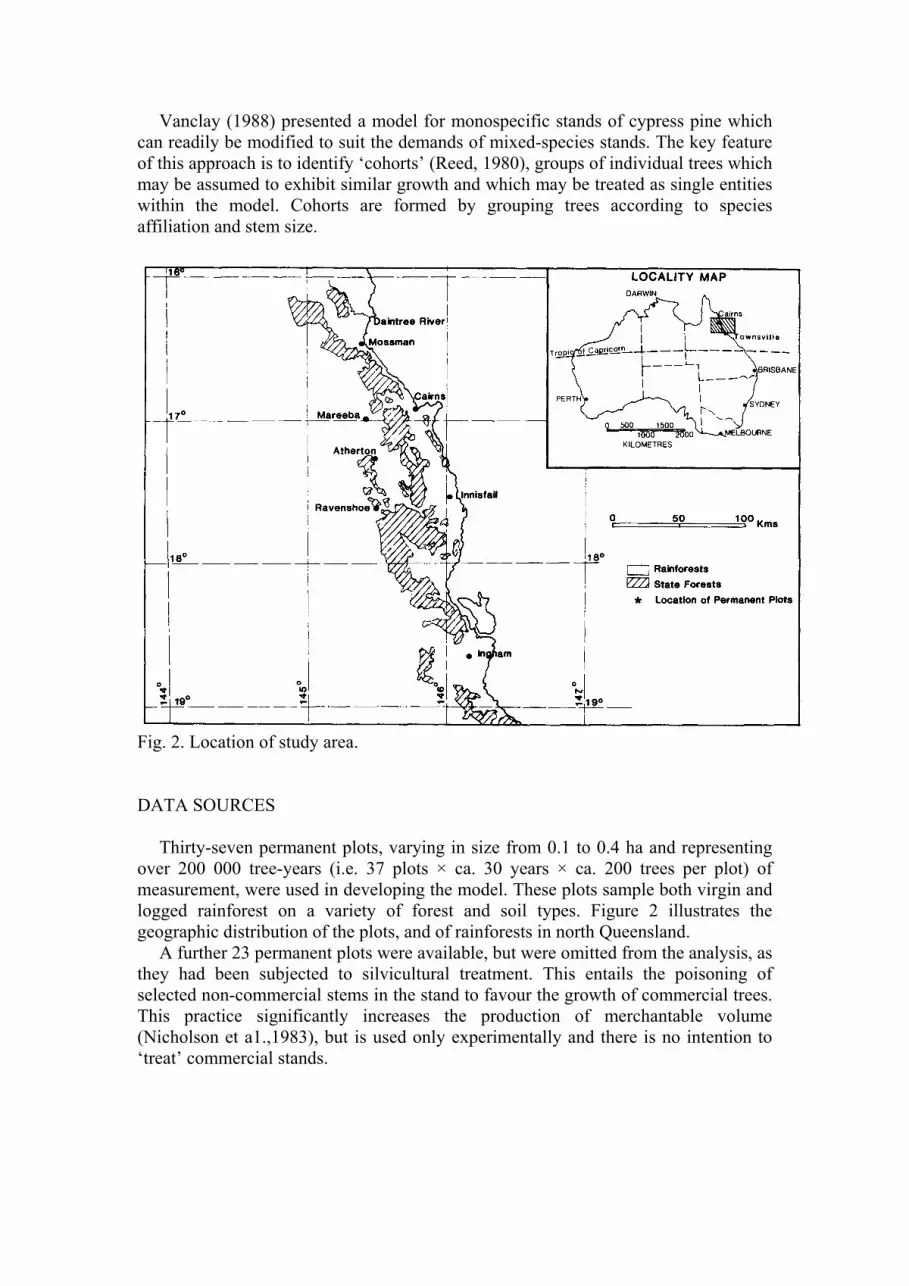
Fig. 2. Location of study area.

DATA SOURCES

Thirty-seven permanent plots, varying in size from 0.1 to 0.4 ha and representing

over 200 000 tree-years (i.e. 37 plots × ca. 30 years × ca. 200 trees per plot) of

measurement, were used in developing the model. These plots sample both virgin and

logged rainforest on a variety of forest and soil types. Figure 2 illustrates the

geographic distribution of the plots, and of rainforests in north Queensland.

A further 23 permanent plots were available, but were omitted from the analysis, as

they had been subjected to silvicultural treatment. This entails the poisoning of

selected non-commercial stems in the stand to favour the growth of commercial trees.

This practice significantly increases the production of merchantable volume

(Nicholson et a1.,1983), but is used only experimentally and there is no intention to

‘treat’ commercial stands.

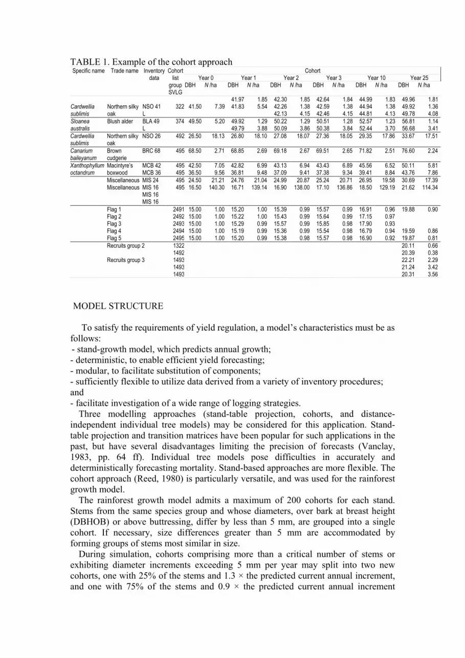
TABLE 1. Example of the cohort approach Cohort

Year 0 Year 1 Year 2 Year 3 Year 10 Year 25 Specific name Trade name Inventory

data Cohort list

group SVLG

DBH N /ha DBH N /ha DBH N /ha DBH N /ha DBH N /ha DBH N /ha

41.97 1.85 42.30 1.85 42.64 1.84 44.99 1.83 49.96 1.81 NSO 41 322 41.50 7.39 41.83 5.54 42.26 1.38 42.59 1.38 44.94 1.38 49.92 1.36

Cardwellia sublimis

Northern silky oak L 42.13 4.15 42.46 4.15 44.81 4.13 49.78 4.08

BLA 49 374 49.50 5.20 49.92 1.29 50.22 1.29 50.51 1.28 52.57 1.23 56.81 1.14 Sloanea australis

Blush alder L 49.79 3.88 50.09 3.86 50.38 3.84 52.44 3.70 56.68 3.41

Cardwellia sublimis

Northern silky oak

NSO 26 492 26.50 18.13 26.80 18.10 27.08 18.07 27.36 18.05 29.35 17.86 33.67 17.51

Canarium baileyanum

Brown cudgerie

BRC 68 495 68.50 2.71 68.85 2.69 69.18 2.67 69.51 2.65 71.82 2.51 76.60 2.24

Xanthophyllum octandrum

Macintyre’s boxwood

MCB 42 MCB 36

495495

42.50 36.50

7.05 9.56

42.82 36.81

6.99 9.48

43.13 37.09

6.94 9.41

43.43 37.38

6.89 9.34

45.56 39.41

6.52 8.84

50.11 43.76

5.81 7.86

Miscellaneous MIS 24 495 24.50 21.21 24.76 21.04 24.99 20.87 25.24 20.71 26.95 19.58 30.69 17.39 Miscellaneous MIS 16

MIS 16 MIS 16

495 16.50 140.30 16.71 139.14 16.90 138.00 17.10 136.86 18.50 129.19 21.62 114.34

Flag 1 2491 15.00 1.00 15.20 1.00 15.39 0.99 15.57 0.99 16.91 0.96 19.88 0.90 Flag 2 2492 15.00 1.00 15.22 1.00 15.43 0.99 15.64 0.99 17.15 0.97 Flag 3 2493 15.00 1.00 15.29 0.99 15.57 0.99 15.85 0.98 17.90 0.93 Flag 4 2494 15.00 1.00 15.19 0.99 15.36 0.99 15.54 0.98 16.79 0.94 19.59 0.86 Flag 5 2495 15.00 1.00 15.20 0.99 15.38 0.98 15.57 0.98 16.90 0.92 19.87 0.81

Recruits group 2 1322 20.11 0.66 1492 20.39 0.38 Recruits group 3 1493 22.21 2.29 1493 21.24 3.42 1493 20.31 3.56

MODEL STRUCTURE

To satisfy the requirements of yield regulation, a model’s characteristics must be as

follows:

- stand-growth model, which predicts annual growth;

- deterministic, to enable efficient yield forecasting;

- modular, to facilitate substitution of components;

- sufficiently flexible to utilize data derived from a variety of inventory procedures;

and

- facilitate investigation of a wide range of logging strategies.

Three modelling approaches (stand-table projection, cohorts, and distance-

independent individual tree models) may be considered for this application. Stand-

table projection and transition matrices have been popular for such applications in the

past, but have several disadvantages limiting the precision of forecasts (Vanclay,

1983, pp. 64 ff). Individual tree models pose difficulties in accurately and

deterministically forecasting mortality. Stand-based approaches are more flexible. The

cohort approach (Reed, 1980) is particularly versatile, and was used for the rainforest

growth model.

The rainforest growth model admits a maximum of 200 cohorts for each stand.

Stems from the same species group and whose diameters, over bark at breast height

(DBHOB) or above buttressing, differ by less than 5 mm, are grouped into a single

cohort. If necessary, size differences greater than 5 mm are accommodated by

forming groups of stems most similar in size.

During simulation, cohorts comprising more than a critical number of stems or

exhibiting diameter increments exceeding 5 mm per year may split into two new

cohorts, one with 25% of the stems and 1.3 × the predicted current annual increment,

and one with 75% of the stems and 0.9 × the predicted current annual increment

(Table 1). This reflects the skewed nature of increment commonly observed in

rainforest stands (Bragg and Henry, 1985). The critical number of stems varies with

stem size, being 20 stems per ha for stems below 40-cm diameter, five stems per ha

for stems exceeding 40-cm diameter, and two stems per ha for stems exceeding the

normal merchantable size (50-100 cm diameter, depending upon species). During the

simulation, the total number of cohorts is maintained below 200 by merging cohorts

with similar diameters and identical species groups.

SPECIES GROUPS

Several hundred tree species are represented in Queensland rainforests (Hyland,

1982), of which more than 100 are of commercial importance. As it is clearly

impractical to develop separate functional relationships for each tree species, some

aggregation is essential. It is expedient to employ three criteria, namely the

volume/size relationship, logging practice, and growth patterns. In the model, species

groups are identified by a four-digit code, SVLG, where S represents the datum source

(0 = inventory, 1 = predicted ingrowth), V indicates the volume relationship to be used

(1 to 4), L indicates the logging rule applicable (1 to 9 inclusive), and G indicates the

growth group. Five growth groups are identified:

(1) commercial species which grow rapidly to a large size;

(2) commercial species which grow slowly to a large size;

(3) commercial species which grow rapidly to a small size;

(4) commercial species which grow slowly to a small size; and

(5) non-commercial species.

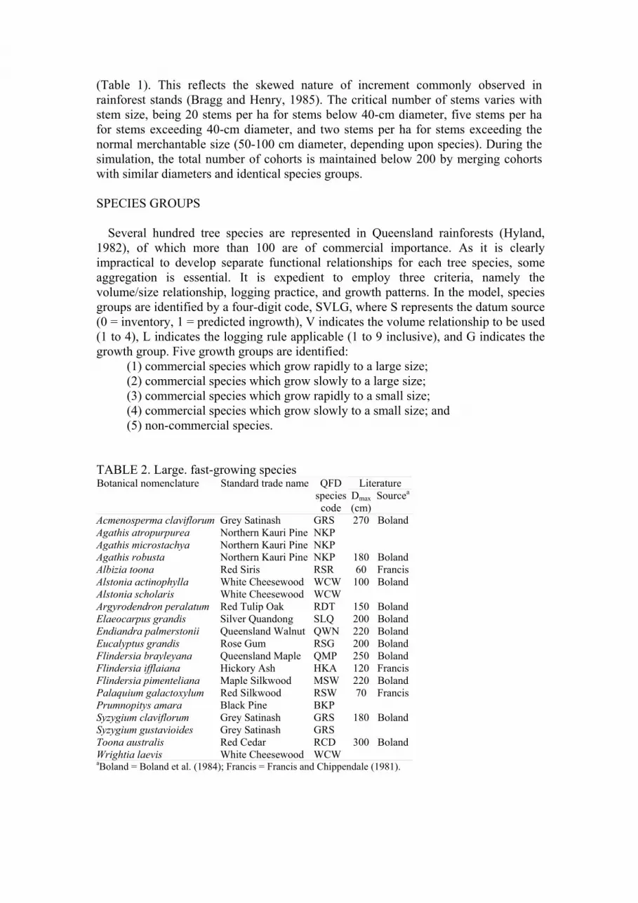
TABLE 2. Large. fast-growing species Literature Botanical nomenclature Standard trade name QFD

species

code

Dmax

(cm)

Sourcea

Acmenosperma claviflorum

Agathis atropurpurea

Agathis microstachya

Grey Satinash

Northern Kauri Pine

Northern Kauri Pine

GRS

NKP

NKP

270 Boland

Agathis robusta Northern Kauri Pine NKP 180 Boland

Albizia toona Red Siris RSR 60 Francis

Alstonia actinophylla

Alstonia scholaris

White Cheesewood

White Cheesewood

WCW

WCW

100 Boland

Argyrodendron peralatum Red Tulip Oak RDT 150 Boland

Elaeocarpus grandis Silver Quandong SLQ 200 Boland

Endiandra palmerstonii Queensland Walnut QWN 220 Boland

Eucalyptus grandis Rose Gum RSG 200 Boland

Flindersia brayleyana Queensland Maple QMP 250 Boland

Flindersia ifflaiana Hickory Ash HKA 120 Francis

Flindersia pimenteliana Maple Silkwood MSW 220 Boland

Palaquium galactoxylum

Prumnopitys amara

Red Silkwood

Black Pine

RSW

BKP

70 Francis

Syzygium claviflorum

Syzygium gustavioides

Grey Satinash

Grey Satinash

GRS

GRS

180 Boland

Toona australis Red Cedar RCD 300 Boland

Wrightia laevis White Cheesewood WCW aBoland = Boland et al. (1984); Francis = Francis and Chippendale (1981).

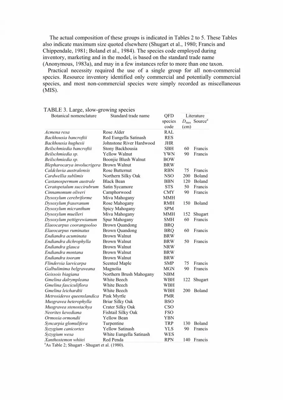
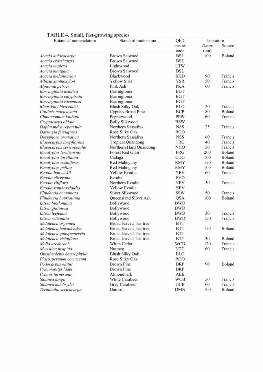
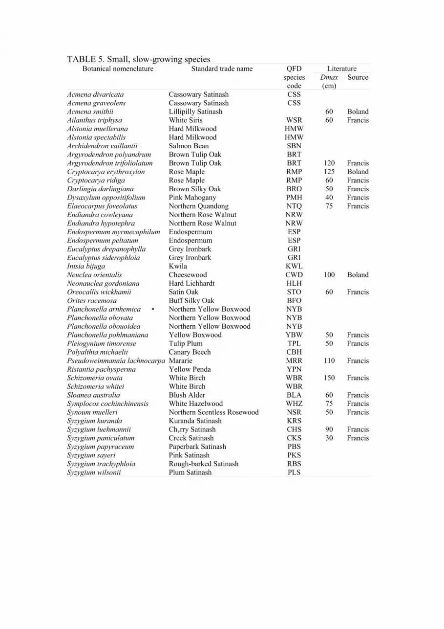
The actual composition of these groups is indicated in Tables 2 to 5. These Tables

also indicate maximum size quoted elsewhere (Shugart et al., 1980; Francis and

Chippendale, 1981; Boland et al., 1984). The species code employed during

inventory, marketing and in the model, is based on the standard trade name

(Anonymous, 1983a), and may in a few instances refer to more than one taxon.

Practical necessity required the use of a single group for all non-commercial

species. Resource inventory identified only commercial and potentially commercial

species, and most non-commercial species were simply recorded as miscellaneous

(MIS).

TABLE 3. Large, slow-growing species Literature Botanical nomenclature Standard trade name QFD

species

code

Dmax

(cm)

Sourcea

Acmena resa

Backhousia bancroftii

Backhousia hughesii

Beilschmiedia bancroftii

Beilschmiedia sp.

Beilschmiedia sp.

Blepharocarya involucrigera

Caldcluvia australensis

Cardwellia sublimis

Castanospermum australe

Ceratopetalum succirubrum

Cinnamomum oliveri

Dysoxylum cerebriforme

Dysoxylum fraseranum

Dysoxylum micranthum

Dysoxylum muelleri

Dysoxylum pettigrewianum

Elaeocarpus coorangooloo

Elaeocarpus ruminatus

Endiandra acuminata

Endiandra dichrophylla

Endiandra glauca

Endiandra montana

Endiandra tooram

Flindersia laevicarpa

Galbulimima belgraveana

Geissois biagiana

Gmelina dalrympleana

Gmelina fasciculiflora

Gmelina leichardtii

Metrosideros queenslandica

Musgravea heterophylla

Musgravea stenostachya

Neorites kevediana

Ormosia ormondii

Syncarpia glomulifera

Syzygium canicortex

Syzygium wesa

Xanthostemon whitei

Rose Alder

Red Eungella Satinash

Johnstone River Hardwood

Stony Backhousia

Yellow Walnut

Boonjie Blush Walnut

Brown Walnut

Rose Butternut

Northern Silky Oak

Black Bean

Satin Sycamore

Camphorwood

Miva Mahogany

Rose Mahogany

Spicy Mahogany

Miva Mahogany

Spur Mahogany

Brown Quandong

Brown Quandong

Brown Walnut

Brown Walnut

Brown Walnut

Brown Walnut

Brown Walnut

Scented Maple

Magnolia

Northern Brush Mahogany

White Beech

White Beech

White Beech

Pink Myrtle

Briar Silky Oak

Crater Silky Oak

Fishtail Silky Oak

Yellow Bean

Turpentine

Yellow Satinash

White Eungella Satinash

Red Penda

RAL

RES

JHR

SBH

YWN

BOW

BRW

RBN

NSO

BBN

STS

CMY

MMH

RMH

SPM

MMH

SMH

BRQ

BRQ

BRW

BRW

NRW

BRW

BRW

SMP

MGN

NBM

WBH

WBH

WBH

PMR

BSO

CSO

FSO

YBN

TRP

YLS

WES

RPN

60

90

75

200

120

50

90

150

152

60

60

50

75

90

122

200

130

90

140

Francis

Francis

Francis

Boland

Boland

Francis

Francis

Boland

Shugart

Francis

Francis

Francis

Francis

Francis

Shugart

Boland

Boland

Francis

Francis aAs Table 2; Shugart - Shugart et al. (1980).

TABLE 4. Small, fast-growing species Literature Botanical nomenclature Standard trade name QFD

species

code

Dmax

(cm)

Source

Acacia aulacocarpa Brown Salwood BSL 100 Boland

Acacia crassicarpa

Acacia implexa

Acacia mangium

Acacia melanoxylon

Brown Salwood

Lightwood

Brown Salwood

Blackwood

BSL

LTW

BSL

BKD

90

Francis

Albizia xanthoxylon Yellow Siris YSR 50 Francis

Alpitonia petriei Pink Ash PKA 60 Francis

Barringtonia asiatica

Barringtonia calyptrata

Barringtonia racemosa

Bleasdalei bleasdalei

Barringtonia

Barringtonia

Barringtonia

Blush Silky Oak

BGT

BGT

BGT

BLO

20

Francis

Callitris macleayana Cypress Brush Pine BCP 80 Boland

Cinnamomum laubatii Pepperwood PPW 60 Francis

Cryptocarya oblata

Daphnandra repandula

Bolly Silkwood

Northern Sassafras

BSW

NSS

25

Francis

Darlingia ferruginea Rose Silky Oak ROO

Doryphora aromatica Northern Sassafras NSS 60 Francis

Elaeocarpus largiflorens Tropical Quandong TRQ 40 Francis

Elaeocarpus sericopetalus Northern Hard Quandong NHQ 50 Francis

Eucalyptus tereticornis Forest Red Gum FRG 200 Boland

Eucalyptus torelliana Cadaga CDG 100 Boland

Eucalyptus resinifera Red Mahogany RMY 150 Boland

Eucalyptus pellita Red Mahogany RMY 100 Boland

Euodia bonwickii Yellow Evodia YEV 60 Francis

Euodia elleryana

Euodia vitiflora

Evodia

Northern Evodia

EVD

NEV

50

Francis

Euodia xanthoxyloides

Flindersia acuminata

Yellow Evodia

Silver Silkwood

YEV

SSW

50

Francis

Flindersia bourjotiana Queensland Silver Ash QSA 100 Boland

Litsea bindoniana

Litsea glutinosa

Litsea leefeana

Bollywood

Bollywood

Bollywood

BWD

BWD

BWD

30

Francis

Litsea reticulata Bollywood BWD 150 Francis

Melaleuca argentea

Melaleuca leucadendra

Broad-leaved Tea-tree

Broad-leaved Tea-tree

BTT

BTT

150

Boland

Melaleuca quinquenervia

Melaleuca viridiflora

Broad-leaved Tea-tree

Broad-leaved Tea-tree

BTT

BTT

30

Boland

Melia azedarach White Cedar WCD 120 Francis

Myristica insipida Nutmeg NTG 60 Francis

Opistheolepis heterophylla

Placospermum coriaceum

Podocarpus elatus

Blush Silky Oak

Rose Silky Oak

Brown Pine

BLO

ROO

BRP

90

Boland

Prumnopitys ladei

Prunus turnerana

Sloanea langii

Brown Pine

Almondbark

White Carabeen

BRP

ALB

WCB

50

Francis

Sloanea macbrydei Grey Carabeen GCB 60 Francis

Terminalia sericocarpa Damson DMN 100 Boland

TABLE 5. Small, slow-growing species Literature Botanical nomenclature Standard trade name QFD

species

code

Dmax

(cm)

Source

Acmena divaricata

Acmena graveolens

Acmena smithii

Cassowary Satinash

Cassowary Satinash

Lillipilly Satinash

CSS

CSS

60

Boland

Ailanthus triphysa White Siris WSR 60 Francis

Alstonia muellerana

Alstonia spectabilis

Archidendron vaillantii

Argyrodendron polyandrum

Argyrodendron trifoliolatum

Hard Milkwood

Hard Milkwood

Salmon Bean

Brown Tulip Oak

Brown Tulip Oak

HMW

HMW

SBN

BRT

BRT

120

Francis

Cryptocarya erythroxylon Rose Maple RMP 125 Boland

Cryptocarya ridiga Rose Maple RMP 60 Francis

Darlingia darlingiana Brown Silky Oak BRO 50 Francis

Dysaxylum oppositifolium Pink Mahogany PMH 40 Francis

Elaeocarpus foveolatus Northern Quandong NTQ 75 Francis

Endiandra cowleyana

Endiandra hypotephra

Endospermum myrmecophilum

Endospermum peltatum

Eucalyptus drepanophylla

Eucalyptus siderophloia

Intsia bijuga

Neuclea orientalis

Northern Rose Walnut

Northern Rose Walnut

Endospermum

Endospermum

Grey Ironbark

Grey Ironbark

Kwila

Cheesewood

NRW

NRW

ESP

ESP

GRI

GRI

KWL

CWD

100

Boland

Neonauclea gordoniana

Oreocallis wickhamii

Hard Lichhardt

Satin Oak

HLH

STO

60

Francis

Orites racemosa

Planchonella arnhemica •

Planchonella obovata

Planchonella obouoidea

Planchonella pohlmaniana

Buff Silky Oak

Northern Yellow Boxwood

Northern Yellow Boxwood

Northern Yellow Boxwood

Yellow Boxwood

BFO

NYB

NYB

NYB

YBW

50

Francis

Pleiogynium timorense Tulip Plum TPL 50 Francis

Polyalthia michaelii

Pseudoweinmannia lachnocarpa

Canary Beech

Mararie

CBH

MRR

110

Francis

Ristantia pachysperma

Schizomeria ovata

Yellow Penda

White Birch

YPN

WBR

150

Francis

Schizomeria whitei

Sloanea australia

White Birch

Blush Alder

WBR

BLA

60

Francis

Symplocos cochinchinensis White Hazelwood WHZ 75 Francis

Synoum muelleri Northern Scentless Rosewood NSR 50 Francis

Syzygium kuranda

Syzygium luehmannii

Kuranda Satinash

Chvrry Satinash

KRS

CHS

90

Francis

Syzygium paniculatum Creek Satinash CKS 30 Francis

Syzygium papyraceum

Syzygium sayeri

Syzygium trachyphloia

Syzygium wilsonii

Paperbark Satinash

Pink Satinash

Rough-barked Satinash

Plum Satinash

PBS

PKS

RBS

PLS

SITE CLASSIFICATION

As rainforests in north Queensland exhibit a considerable variation in growth rate

and timber production, it is necessary to assess site productivity. To facilitate efficient

site assessment during routine inventory, it is desirable to identify quality classes, and

an objective means of appraisal.

The 37 permanent plots were ranked according to their past basal area and volume

increments, and local field-staff attempted to identify meaningful plot attributes

correlated with rank. They identified four factors which may influence and indicate

volume increment: soil parent material; species composition; standing volume; and

log length. The appraisal scheme assigned points to each attribute, producing a total

score ranging from 1 to 30. The point scores for each attribute were initially

subjectively assigned, and were iteratively refined until the total scores allocated to

each of the permanent plots reflected their ranking.

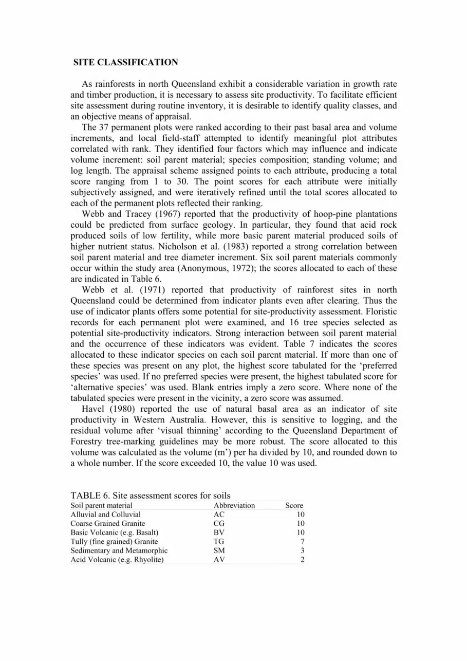
Webb and Tracey (1967) reported that the productivity of hoop-pine plantations

could be predicted from surface geology. In particular, they found that acid rock

produced soils of low fertility, while more basic parent material produced soils of

higher nutrient status. Nicholson et al. (1983) reported a strong correlation between

soil parent material and tree diameter increment. Six soil parent materials commonly

occur within the study area (Anonymous, 1972); the scores allocated to each of these

are indicated in Table 6.

Webb et al. (1971) reported that productivity of rainforest sites in north

Queensland could be determined from indicator plants even after clearing. Thus the

use of indicator plants offers some potential for site-productivity assessment. Floristic

records for each permanent plot were examined, and 16 tree species selected as

potential site-productivity indicators. Strong interaction between soil parent material

and the occurrence of these indicators was evident. Table 7 indicates the scores

allocated to these indicator species on each soil parent material. If more than one of

these species was present on any plot, the highest score tabulated for the ‘preferred

species’ was used. If no preferred species were present, the highest tabulated score for

‘alternative species’ was used. Blank entries imply a zero score. Where none of the

tabulated species were present in the vicinity, a zero score was assumed.

Havel (1980) reported the use of natural basal area as an indicator of site

productivity in Western Australia. However, this is sensitive to logging, and the

residual volume after ‘visual thinning’ according to the Queensland Department of

Forestry tree-marking guidelines may be more robust. The score allocated to this

volume was calculated as the volume (m’) per ha divided by 10, and rounded down to

a whole number. If the score exceeded 10, the value 10 was used.

TABLE 6. Site assessment scores for soils Soil parent material Abbreviation Score

Alluvial and Colluvial AC 10

Coarse Grained Granite CG 10

Basic Volcanic (e.g. Basalt) BV 10

Tully (fine grained) Granite TG 7

Sedimentary and Metamorphic SM 3

Acid Volcanic (e.g. Rhyolite) AV 2

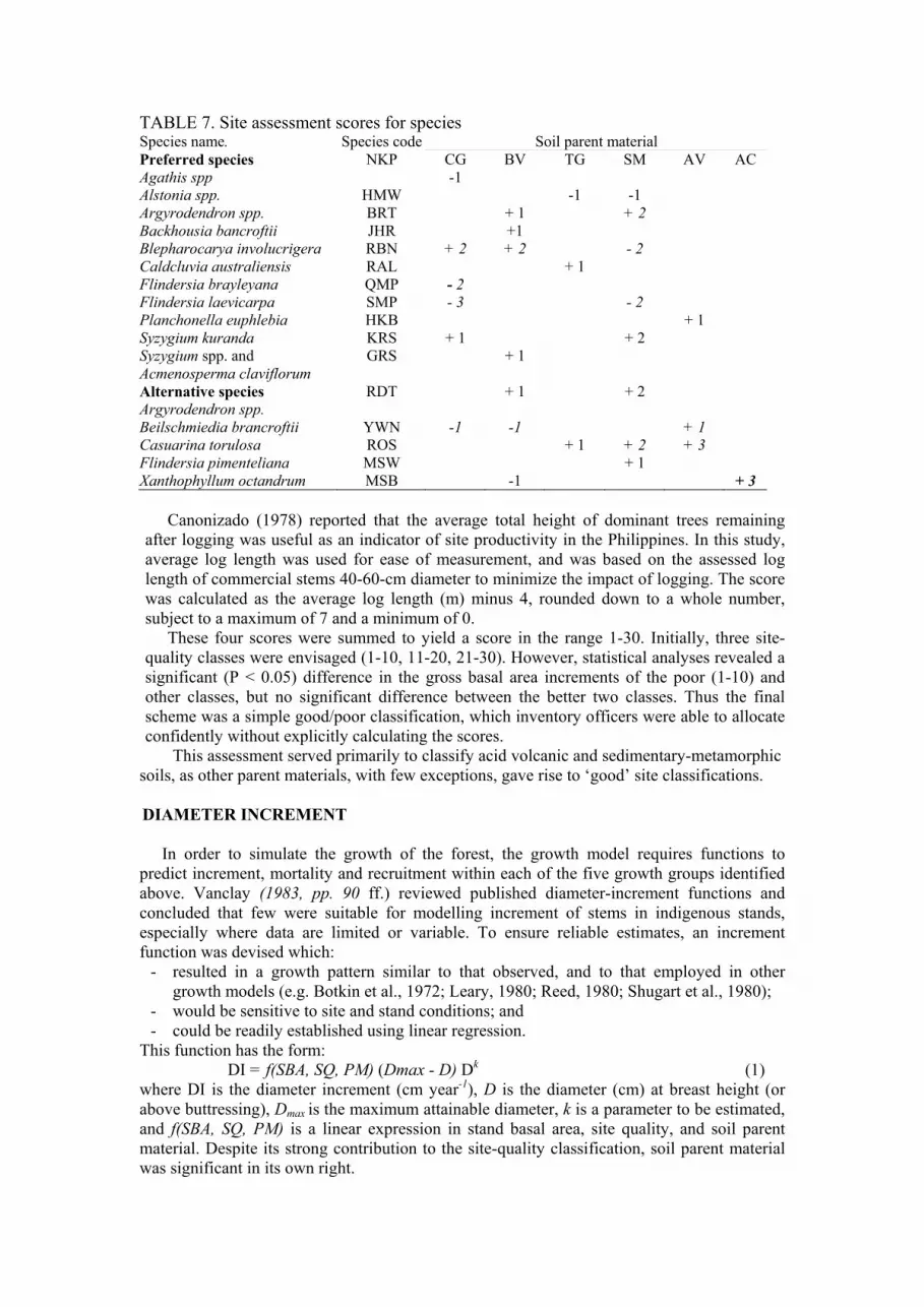
TABLE 7. Site assessment scores for species Species name. Species code Soil parent material

Preferred species

Agathis spp

NKP CG

-1

BV TG SM AV AC

Alstonia spp. HMW -1 -1

Argyrodendron spp. BRT + 1 + 2

Backhousia bancroftii JHR +1

Blepharocarya involucrigera RBN + 2 + 2 - 2

Caldcluvia australiensis RAL + 1

Flindersia brayleyana QMP - 2

Flindersia laevicarpa SMP - 3 - 2

Planchonella euphlebia HKB + 1

Syzygium kuranda KRS + 1 + 2

Syzygium spp. and

Acmenosperma claviflorum

GRS + 1

Alternative species

Argyrodendron spp.

RDT + 1 + 2

Beilschmiedia brancroftii YWN -1 -1 + 1

Casuarina torulosa ROS + 1 + 2 + 3

Flindersia pimenteliana MSW + 1

Xanthophyllum octandrum MSB -1 + 3

Canonizado (1978) reported that the average total height of dominant trees remaining

after logging was useful as an indicator of site productivity in the Philippines. In this study,

average log length was used for ease of measurement, and was based on the assessed log

length of commercial stems 40-60-cm diameter to minimize the impact of logging. The score

was calculated as the average log length (m) minus 4, rounded down to a whole number,

subject to a maximum of 7 and a minimum of 0.

These four scores were summed to yield a score in the range 1-30. Initially, three site-

quality classes were envisaged (1-10, 11-20, 21-30). However, statistical analyses revealed a

significant (P < 0.05) difference in the gross basal area increments of the poor (1-10) and

other classes, but no significant difference between the better two classes. Thus the final

scheme was a simple good/poor classification, which inventory officers were able to allocate

confidently without explicitly calculating the scores.

This assessment served primarily to classify acid volcanic and sedimentary-metamorphic

soils, as other parent materials, with few exceptions, gave rise to ‘good’ site classifications.

DIAMETER INCREMENT

In order to simulate the growth of the forest, the growth model requires functions to

predict increment, mortality and recruitment within each of the five growth groups identified

above. Vanclay (1983, pp. 90 ff.) reviewed published diameter-increment functions and

concluded that few were suitable for modelling increment of stems in indigenous stands,

especially where data are limited or variable. To ensure reliable estimates, an increment

function was devised which:

- resulted in a growth pattern similar to that observed, and to that employed in other

growth models (e.g. Botkin et al., 1972; Leary, 1980; Reed, 1980; Shugart et al., 1980);

- would be sensitive to site and stand conditions; and

- could be readily established using linear regression.

This function has the form:

DI = f(SBA, SQ, PM) (Dmax - D) Dk (1)

where DI is the diameter increment (cm year-1), D is the diameter (cm) at breast height (or

above buttressing), Dmax is the maximum attainable diameter, k is a parameter to be estimated,

and f(SBA, SQ, PM) is a linear expression in stand basal area, site quality, and soil parent

material. Despite its strong contribution to the site-quality classification, soil parent material

was significant in its own right.

Attainable diameter

As trees become very large, irrespective of their general health and vigour, their diameter

increment declines as a consequence of increasing respiratory demands relative to the

effective photosynthetic area. Thus, for most tree species it is appropriate to identify a

maximum attainable diameter (Dmax), the size which a given species on a nominated site can

barely attain.

The Dmax can be estimated using statistical analyses where sufficient data are available.

However, in rainforests (even virgin stands), very large stems occur infrequently, and few

data exist for these stems. Thus it is expedient to subjectively determine the Dmax for each

growth group, based on inspection of available data, relevant literature (Shugart et al., 1980;

Francis and Chippendale, 1981; Boland et al., 1984) and local knowledge. The variation in

Dmax on the different soil parent materials is due both to different growth habits of individual

species, and to the different species composition of growth groups.

Growth pattern

The predicted growth pattern is determined largely by the parameter k in Equation (1).

This parameter may be expected to take a value between 0 and 1, depending upon the growth

habits of the species comprising the group. Graphical analysis revealed that for most groups

a value of 0.667 appeared to be appropriate. Statistical analysis revealed that, for groups 1, 2

and 5 on all sites, the estimated values were very close to and not significantly (P < 0.05)

different from 0.667, which was consequently adopted. Slightly different values were

obtained for growth groups 3 and 4.

Growth rates

In Equation (1), the predicted rate of growth is determined by the expression f(SBA, SQ,

PM), which was determined by ordinary least-squares linear regression. Because of the vast

amount of data, and the disproportionate representation of smaller size classes, and to

facilitate graphical analyses of the residuals, the data were grouped into site quality, soil

parent material and 5 cm-diameter cells. Some cells were further grouped to enable the

estimation of the variance within each cell. The mean diameter of each cell was used in the

analysis, and site quality and soil parent material were included as dummy (0, 1) variables.

Linear regression, weighted by the inverse of the variance, produced the following results

(all parameters significant at P< 0.05 or better throughout the paper):

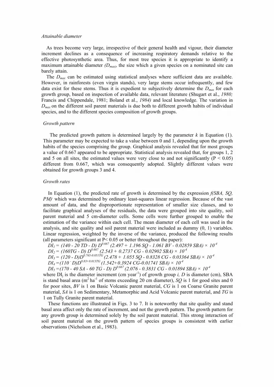
DI1 = (140 - 20 TD - D) D0.667 (2.497 + 1.196 SQ - 1.061 BV - 0.02859 SBA) × 10-4

DI2 = (160TG - D) D0.667 (2.543 + 0.2737 CG - 0.02902 SBA) × 10-4

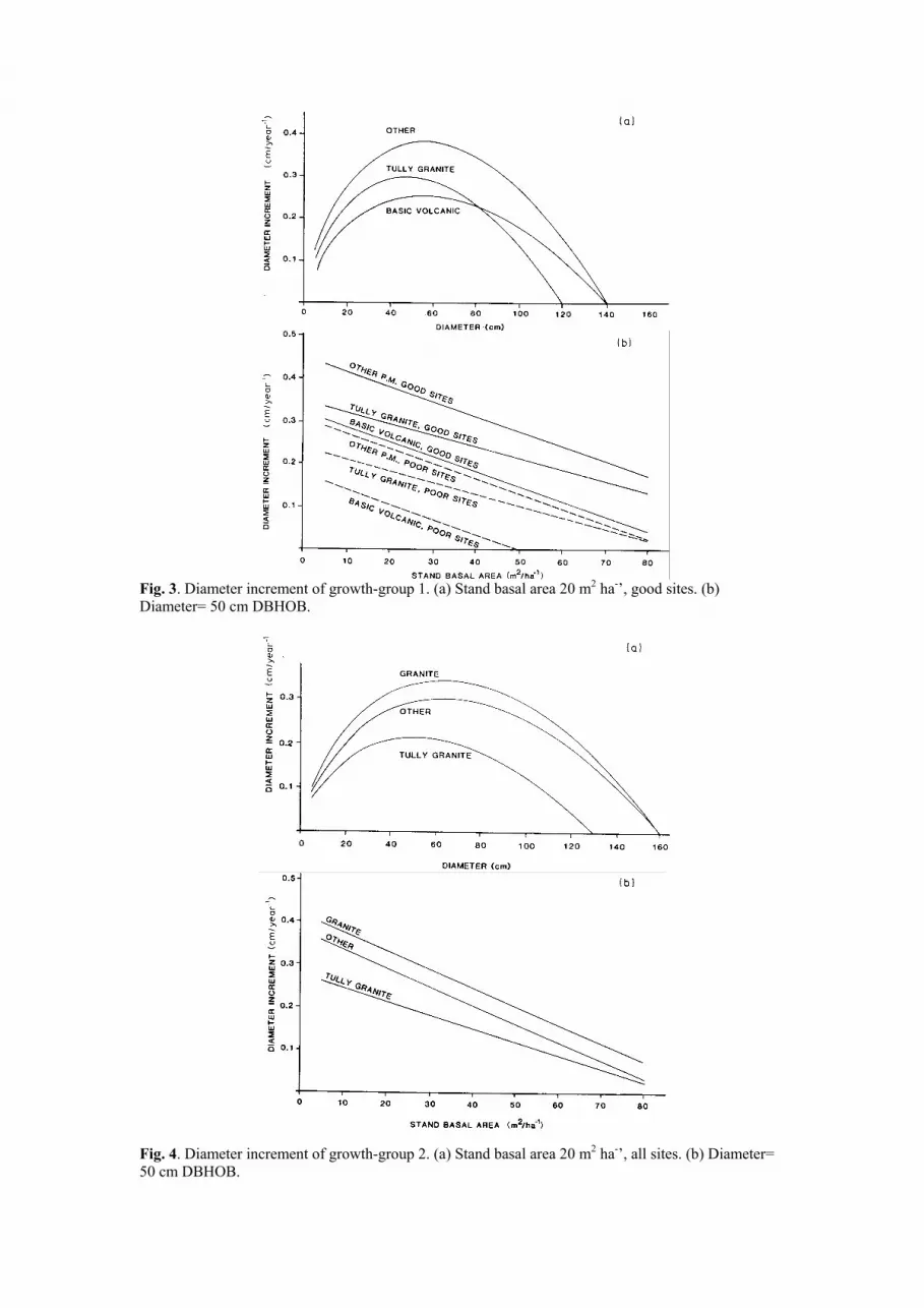
DI3 = (120 - D)D0.765-0.051TG (2.478 + 1.055 SQ - 0.8328 CG - 0.03364 SBA) × 10-4

DI4 =(110 - D)D0.83+0.013TG (1.542+0.3924 CG-0.01741 SBA) × 10-4

DI5 =(170 - 40 SA - 60 TG - D) D0.667 (2.076 - 0.3831 CG - 0.01894 SBA) × 10-4

where DIj is the diameter increment (cm year-1) of growth group i, D is diameter (cm), SBA

is stand basal area (m2 ha-1 of stems exceeding 20 cm diameter), SQ is 1 for good sites and 0

for poor sites, BV is 1 on Basic Volcanic parent material, CG is 1 on Coarse Granite parent

material, SA is 1 on Sedimentary, Metamorphic and Acid Volcanic parent material, and TG is

1 on Tully Granite parent material.

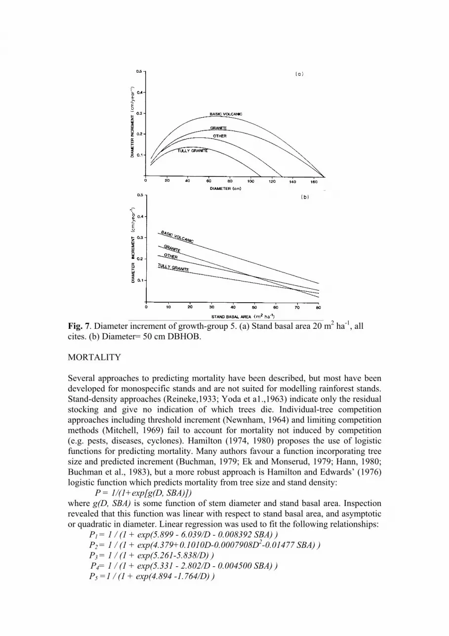
These functions are illustrated in Figs. 3 to 7. It is noteworthy that site quality and stand

basal area affect only the rate of increment, and not the growth pattern. The growth pattern for

any growth group is determined solely by the soil parent material. This strong interaction of

soil parent material on the growth pattern of species groups is consistent with earlier

observations (Nicholson et al., 1983).

Fig. 3. Diameter increment of growth-group 1. (a) Stand basal area 20 m2 ha-’, good sites. (b)

Diameter= 50 cm DBHOB.

Fig. 4. Diameter increment of growth-group 2. (a) Stand basal area 20 m2 ha-’, all sites. (b) Diameter=

50 cm DBHOB.

Fig. 5. Diameter increment of growth-group 3. (a) Stand basal area 20 m2 ha’, good sites. (b)

Diameter= 50 cm DBHOB.

Fig. 6. Diameter increment of growth-group 4. (a) Stand basal area 20 m2 ha-1, all sites. (b) Diameter= 50 cm DBHOB.

Fig. 7. Diameter increment of growth-group 5. (a) Stand basal area 20 m

2 ha

-1, all

cites. (b) Diameter= 50 cm DBHOB.

MORTALITY

Several approaches to predicting mortality have been described, but most have been

developed for monospecific stands and are not suited for modelling rainforest stands.

Stand-density approaches (Reineke,1933; Yoda et a1.,1963) indicate only the residual

stocking and give no indication of which trees die. Individual-tree competition

approaches including threshold increment (Newnham, 1964) and limiting competition

methods (Mitchell, 1969) fail to account for mortality not induced by competition

(e.g. pests, diseases, cyclones). Hamilton (1974, 1980) proposes the use of logistic

functions for predicting mortality. Many authors favour a function incorporating tree

size and predicted increment (Buchman, 1979; Ek and Monserud, 1979; Hann, 1980;

Buchman et al., 1983), but a more robust approach is Hamilton and Edwards’ (1976)

logistic function which predicts mortality from tree size and stand density:

P = 1/(1+exp[g(D, SBA)])

where g(D, SBA) is some function of stem diameter and stand basal area. Inspection

revealed that this function was linear with respect to stand basal area, and asymptotic

or quadratic in diameter. Linear regression was used to fit the following relationships:

P1 = 1 / (1 + exp(5.899 - 6.039/D - 0.008392 SBA) )

P2 = 1 / (1 + exp(4.379+0.1010D-0.0007908D2-0.01477 SBA) )

P3 = 1 / (1 + exp(5.261-5.838/D) )

P4= 1 / (1 + exp(5.331 - 2.802/D - 0.004500 SBA) )

P5 =1 / (1 + exp(4.894 -1.764/D) )

where Pi is the annual probability of mortality within growth-group i, D is diameter

(cm, breast high or above buttress, over bark) and SBA is stand basal area (m2 ha

-1 of

stems exceeding 20 cm diameter) .

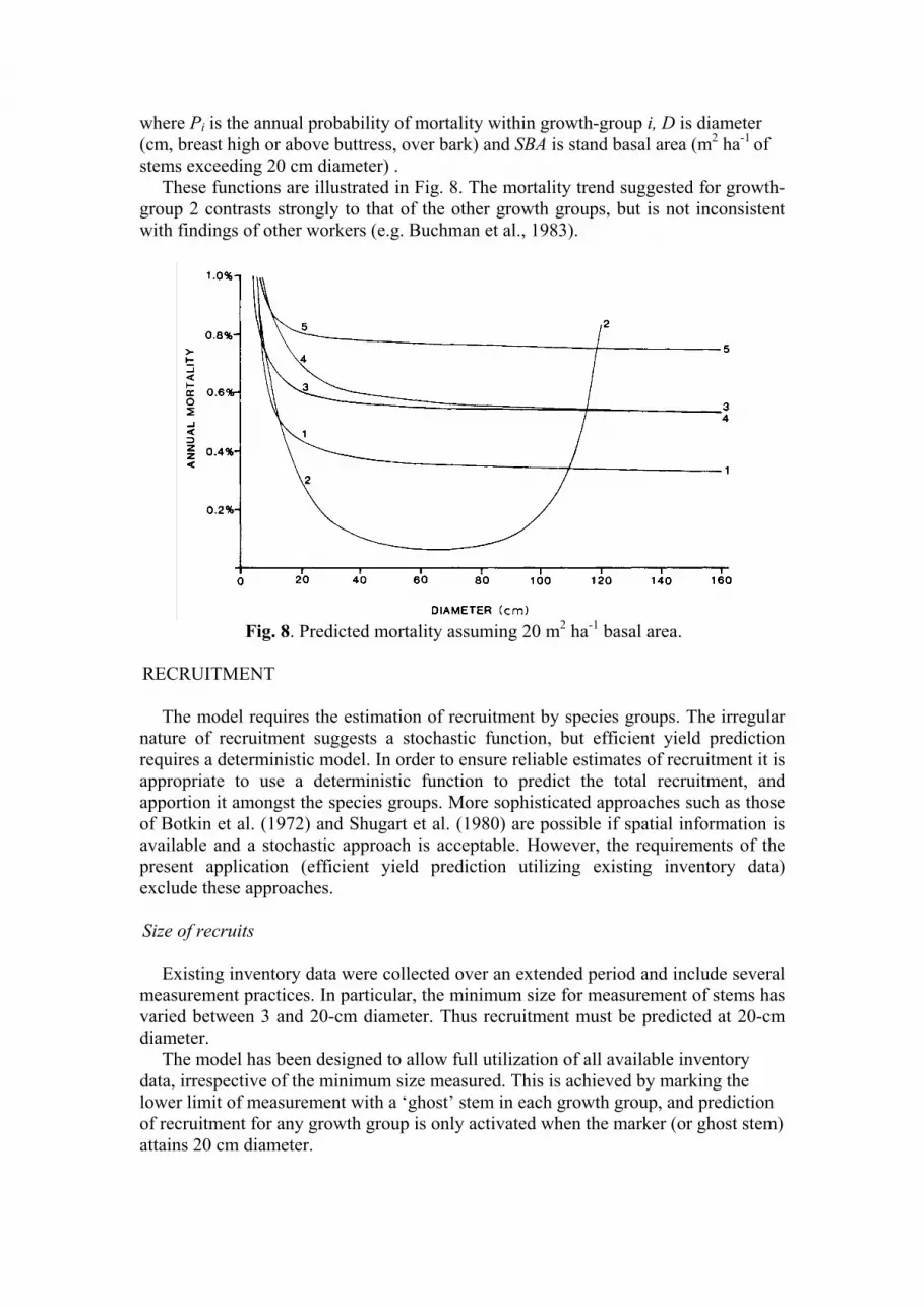
These functions are illustrated in Fig. 8. The mortality trend suggested for growth-

group 2 contrasts strongly to that of the other growth groups, but is not inconsistent

with findings of other workers (e.g. Buchman et al., 1983).

Fig. 8. Predicted mortality assuming 20 m

2 ha

-1 basal area.

RECRUITMENT

The model requires the estimation of recruitment by species groups. The irregular

nature of recruitment suggests a stochastic function, but efficient yield prediction

requires a deterministic model. In order to ensure reliable estimates of recruitment it is

appropriate to use a deterministic function to predict the total recruitment, and

apportion it amongst the species groups. More sophisticated approaches such as those

of Botkin et al. (1972) and Shugart et al. (1980) are possible if spatial information is

available and a stochastic approach is acceptable. However, the requirements of the

present application (efficient yield prediction utilizing existing inventory data)

exclude these approaches.

Size of recruits

Existing inventory data were collected over an extended period and include several

measurement practices. In particular, the minimum size for measurement of stems has

varied between 3 and 20-cm diameter. Thus recruitment must be predicted at 20-cm

diameter.

The model has been designed to allow full utilization of all available inventory

data, irrespective of the minimum size measured. This is achieved by marking the

lower limit of measurement with a ‘ghost’ stem in each growth group, and prediction

of recruitment for any growth group is only activated when the marker (or ghost stem)

attains 20 cm diameter.

Amount of recruitment

Graphical inspection of the data suggested that recruitment was linearly related to

stand basal area and correlated with site quality. The total amount of recruitment was

predicted as:

N = 5.466 -0.06469 SBA +1.013 SQ

where N is the number of recruits (stems ha-1 year

-1 at 20 cm diameter), SBA is stand

basal area (m’ ha -1 of stems exceeding 20-cm diameter), and SQ is 1 on good sites

and 0 on poor sites. On average, recruitment does not exceed 6.5 stems ha-1 year

-1, and

does not occur where stand density exceeds 100 and 85 m2 ha

-1 basal area on good and

poor sites, respectively.

Composition of recruitment

It is important to correctly predict the composition of recruitment by growth group,

as it determines the predicted growth rates and may influence stand basal area.

Logging and volume groups only become important once the recruited stems reach

commercial size, and at this stage warning messages are printed to caution the user

against placing too much reliance upon results derived from stands comprising a

significant proportion of predicted recruitment.

The composition by growth groups can be predicted in two ways. One approach is

to allocate recruits to growth groups according to the current stand composition.

Although the stand composition will be a major determinant of the composition of

seedlings, this approach ignores stand density, a major factor determining recruitment

through its affect on light intensity. An alternative approach is to predict the

proportion of recruitment in each growth group by some function of stand condition.

Stand basal area, composition and site quality may all influence the composition of

recruitment, but no relationship between composition of recruitment and soil parent

material could be detected. As a proportion (of total recruitment) is being predicted, it

is appropriate to use a logistic function (Hamilton, 1974):

Pi = 1 - 1 / (1 + exp [ h (SBA, Bi, SQ)] )

where PI is the proportion of the total recruitment as growth group i, and h (sBA, Bi,

SQ) is some linear function of total stand basal area, basal area of growth group i and

site quality. It is necessary to use the basal area of each growth group rather than the

number of stems as some inventory data are derived from horizontal point sampling

(sampling with probability proportional to size) (Husch et al., 1982, p. 220) in which

the presence or absence of a single small stem may give rise to a large difference in

the estimated number of stems.

The following functions were derived by linear regression:

P1 = 1 - 1 / (1 + exp(-2.407 -0.005608 SBA +0.01105B1 +0.00464B1 SQ) )

P2 = 1 -1 / (1 + exp(-2.572 -0.006756 SBA +0.11800B2 -0.06434B2 SQ) )

P3 = 1 - 1 / (1 + exp(-1.761-0.008240 SBA -0.08076B3 +0.16610B3 SQ) )

P4 = 1 - 1 / (1 + exp(-2.440 -0.010609 SBA +0.16470B4 -0.06230B4 SQ) )

P5 = 1 - 1 / (1 + exp(-0.655 -0.024960 SBA +0.10630B5 - 0.02621B5 SQ) )

where Pi is the proportion of the total recruitment as growth group i, SBA is stand

basal area (m

2 ha

-1 of stems exceeding 20-cm diameter), B1, B2, ..., B5 are the basal

areas of growth groups 1 to 5, respectively, and SQ is 1 on good sites and 0 on poor

sites.

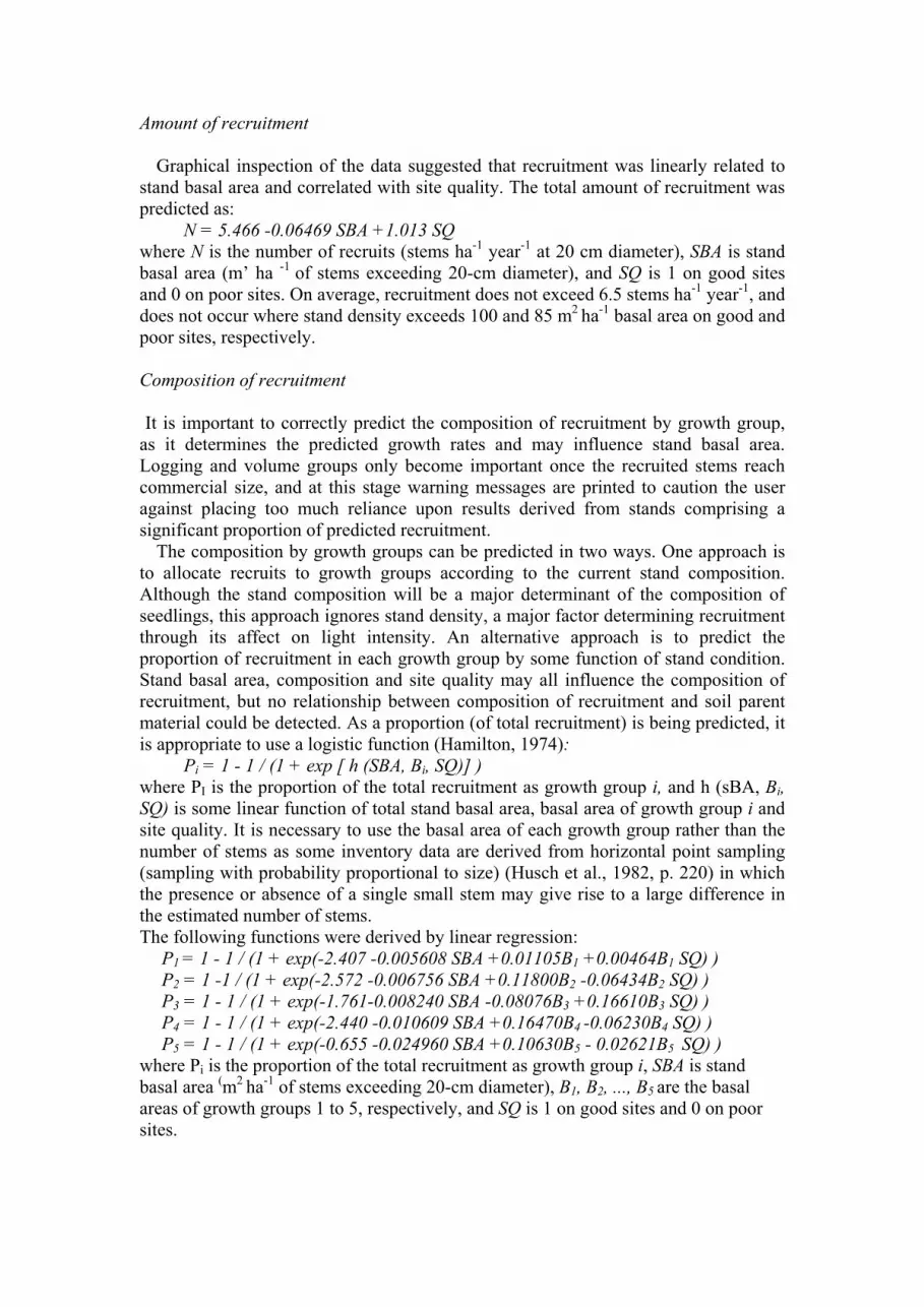
Fig. 9. Recruitment at 20-cm DBH (stems ha -1 year

-1) .

To ensure that these estimated proportions summed to exactly 1.0, the proportions

were standardized:

Pi =Pi / (P1 +P2 +P3 +P4 +P5)

Figure 9 illustrates how recruitment varies in response to changing stand

composition and density.

Logging groups may be allocated to recruits according to the composition of the

corresponding stand fraction, based on numbers of stems rather than basal area, to

ensure that useless veteran trees do not exert a disproportionate effect.

Thus, for example, if it is determined that 5% of the growth-group 1 stems in the

existing stand are useless (logging-group 9), then 5% of the predicted growth-group 1

recruits will be assigned to that category.

A similar procedure can be followed to determine the volume group. However, this

is greatly simplified as volume group is usually uniquely determined by logging

group and growth group.

DISCUSSION

Formal validation of the model has not yet been attempted, but inspection reveals

that the model forecasts stand dynamics generally in accordance with available data

and expectations, even over very long intervals.

Strengths of the model

This growth model represents a considerable advance on previous rainforest yield

prediction models (Higgins, 1977; Bragg and Henry, 1985). Important advances

include the identification of growth groups based on growth characteristics, the

recognition of the influence of stand density on all aspects of stand dynamics, the

explicit identification of a maximum attainable size, an attempt to quantify the site

productivity (by site classification and identification of soil parent material), and the

recognition that stand composition may influence the composition of recruitment.

The advantage in recognising a maximum attainable diameter is that it ensures that

diameter increments cannot be overestimated for the larger trees being modelled, thus

ensuring a robust model.

The model distinguishes stems actually measured during inventory from - those

predicted by the model as recruitment. This serves to warn the user of diminishing

precision of forecasts during long simulations. A weakness inherent in many other

approaches, particularly stand-table projection approaches (e.g. Adams and Ek, 1974)

and matrix approaches (e.g. Usher, 1966) is that predicted recruitment is not

distinguished and the user is not explicitly warned of unrealistically long projections.

Weaknesses of the model

A number of weaknesses in the growth model can be identified. Five growth

groups were identified largely on the basis of growth characteristics, except for the

non-commercial group necessary for practical reasons. Ideally, growth groups should

be formed solely on the basis of growth rate, growth pattern and regeneration

strategy, as commercial criteria may be accommodated in the volume and logging

groups. However, practical difficulties limit the extent to which this can be done.

Existing resource inventory data contain the specific identity of all commercial and

potentially commercial species, but most of the noncommercial species are simply

identified as miscellaneous (MIS). In future inventories, it may be possible to identify

some additional species or species groups, but it is considered impossible to reliably

identify all non-commercial species during resource inventory. A viable solution may

be to identify a number of groups of non-commercial species according to their

growth habit.

It has long been recognised that the productive potential of any forest depends

upon, among other factors, the site productivity. Soil parent material has been

recognised as an important factor for some time (Anonymous, 1981; Nicholson et al.,

1983; Bragg and Henry, 1985), but reflects only part of the site factors. The good/poor

site classification introduced here represents a first attempt to assess site productivity.

Its scope is greatly restricted by its relatively subjective nature, and by the presence of

only two classes. More research is required to establish a more objective and

quantitative assessment procedure.

The model assumes that the merchantability of stems does not change over time.

Thus, if a stem was deemed merchantable at the time of inventory, then it is assumed

to remain merchantable throughout the simulation. Although it seems reasonable that

this should hold for the majority of stems, insufficient data exist to confirm or reject

this assumption.

Prediction of recruitment at 20-cm diameter is less than desirable from a modelling

viewpoint, but is necessary to enable forecasts using all available inventory data.

Some of the functions employed are somewhat simplistic, but these generalizations

are imposed by the available data. For example, the mortality functions allow no

interaction between stand basal area and tree size. Such interaction may exist, but

cannot be detected in the data currently available. In order to detect any such subtle

interactions, more data must be collected.

Implications of the model

The model indicates that rainforest can be managed for timber production using

selection logging over long periods, without significantly altering the species

composition of the stand. This is consistent with previously published findings

(Anonymous, 1983b; Caulfield, 1983).

The model also enables an objective evaluation of the tree-marking guidelines.

These are used by field staff to ensure consistently high standards of forest

management, and encompass several objectives including maintaining the diversity,

and increasing the productivity of the forest (Anonymous, 1981b). To facilitate this

analysis, we assume that the primary objective of forest management is to maximize

timber volume production, that the standing basal area of the forest is held relatively

constant over time, and that there is no social time preference (i.e. future volumes are

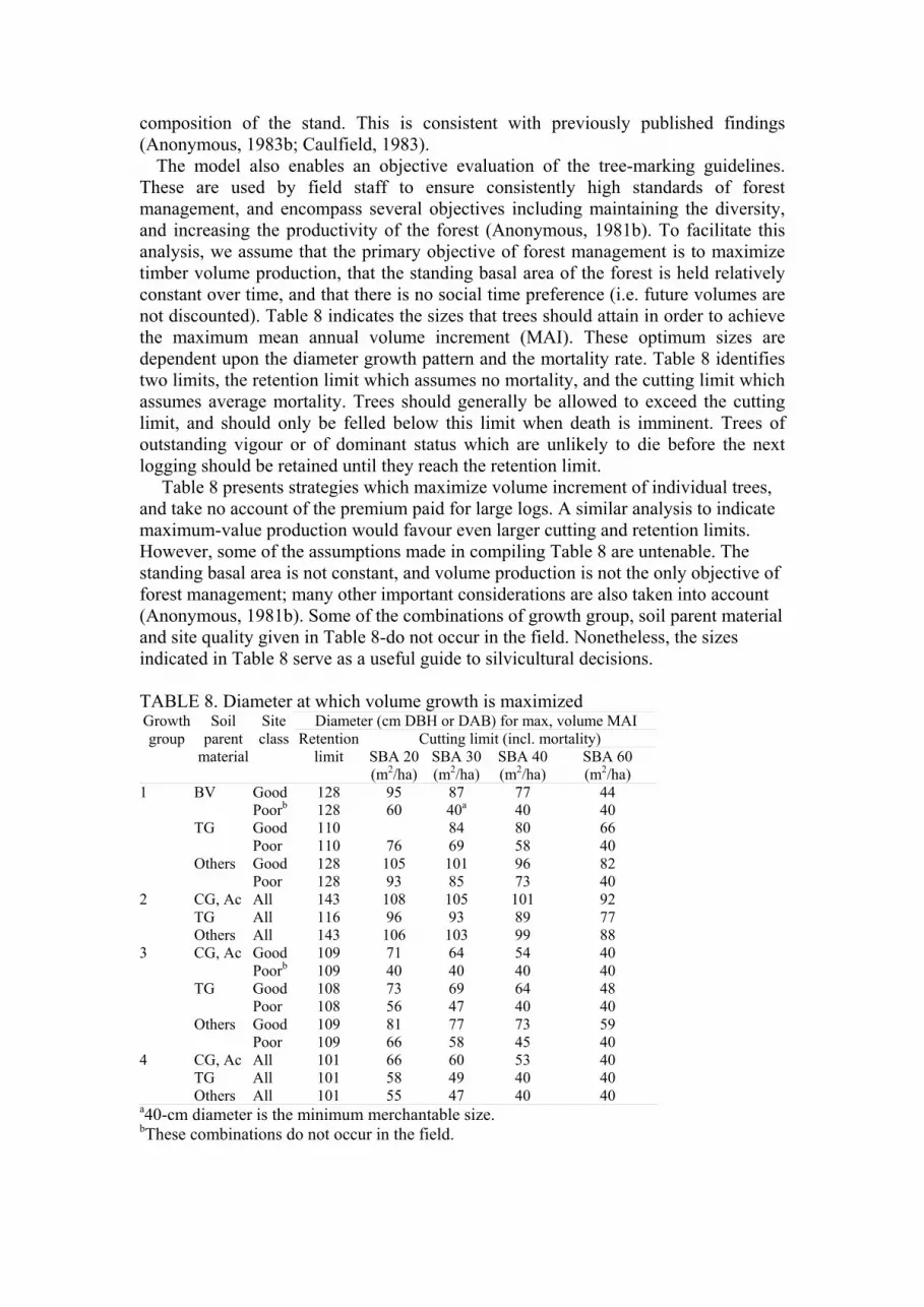
not discounted). Table 8 indicates the sizes that trees should attain in order to achieve

the maximum mean annual volume increment (MAI). These optimum sizes are

dependent upon the diameter growth pattern and the mortality rate. Table 8 identifies

two limits, the retention limit which assumes no mortality, and the cutting limit which

assumes average mortality. Trees should generally be allowed to exceed the cutting

limit, and should only be felled below this limit when death is imminent. Trees of

outstanding vigour or of dominant status which are unlikely to die before the next

logging should be retained until they reach the retention limit.

Table 8 presents strategies which maximize volume increment of individual trees,

and take no account of the premium paid for large logs. A similar analysis to indicate

maximum-value production would favour even larger cutting and retention limits.

However, some of the assumptions made in compiling Table 8 are untenable. The

standing basal area is not constant, and volume production is not the only objective of

forest management; many other important considerations are also taken into account

(Anonymous, 1981b). Some of the combinations of growth group, soil parent material

and site quality given in Table 8-do not occur in the field. Nonetheless, the sizes

indicated in Table 8 serve as a useful guide to silvicultural decisions.

TABLE 8. Diameter at which volume growth is maximized Diameter (cm DBH or DAB) for max, volume MAI

Cutting limit (incl. mortality)

Growth

group

Soil

parent

material

Site

class Retention

limit SBA 20

(m2/ha)

SBA 30

(m2/ha)

SBA 40

(m2/ha)

SBA 60

(m2/ha)

1 BV Good 128 95 87 77 44

Poorb 128 60 40a 40 40

TG Good 110 84 80 66

Poor 110 76 69 58 40

Others Good 128 105 101 96 82

Poor 128 93 85 73 40

2 CG, Ac All 143 108 105 101 92

TG All 116 96 93 89 77

Others All 143 106 103 99 88

3 CG, Ac Good 109 71 64 54 40

Poorb 109 40 40 40 40

TG Good 108 73 69 64 48

Poor 108 56 47 40 40

Others Good 109 81 77 73 59

Poor 109 66 58 45 40

4 CG, Ac All 101 66 60 53 40

TG All 101 58 49 40 40

Others All 101 55 47 40 40 a40-cm diameter is the minimum merchantable size. bThese combinations do not occur in the field.

CONCLUSION

This model has provided an objective basis for appraising management decisions,

and for determining the sustainable yield and allowable cut of Queensland’s northern

rainforests.

Careful selection of component functions has ensured a robust model which

provides realistic forecasts for a diverse range of forest types and inventory data.

Standard analytical techniques including graphical inspection, weighted linear

regression and inspection of residuals were used in developing the model.

This approach may be applicable to other mixed species forests, particularly

rainforests in other tropical countries.

ACKNOWLEDGEMENTS

I am indebted to the many officers of the Queensland Department of Forestry who

participated in the collection of data and the compilation of the database, to R.A.

Preston and I.J. Robb for devising the site assessment procedure, to S.J. Dansie, D.I.

Nicholson, R.A. Preston and E.J. Rudder for suggesting the composition of the growth

groups, to N.B. Henry for his assistance in developing the diameter increment

functions, and to E.J. Rudder for checking the botanical nomenclature. Permission of

the Department of Forestry to publish this paper is acknowledged.

REFERENCES

Adams, D.M. and Ek, A.R., 1974. Optimizing the management of uneven-aged forest

stands. Can. J. For. Res., 4: 274-287.

Anonymous, 1972. 1: 250 000 Geological series - Explanatory notes. Australian

Government Publishing Service, Canberra, A.C.T.

Anonymous, 1979. A generalized forest growth projection system applied to the Lake

States region. USDA For. Serv. Gen. Tech. Rep. NC-49,96 pp.

Anonymous, 1981a. Rainforest increment studies. Queensl. Dep. For. Res. Rep., 3:

63-64. Anonymous, 1981b. Timber production from North Queensland’s

rainforests. Position paper issued by the Queensland Department of Forestry,

Brisbane, Qld., 28 pp.

Anonymous, 1983a. Nomenclature of Australian timbers. Australian Standard 2543-

1983, Standards Association of Australia, Sydney N.S.W., 62 pp.

Anonymous, 1983b. Rainforest Research in North Queensland. Position paper issued

by the Queensland Department of Forestry, Brisbane, Qld., 52 pp.

Boland, D.J., Brooker, M.I.H., Chippendale, G.M., Hall, N., Hyland, B.P.M.,

Johnston, R.D.,

Kleinig, D.A. and Turner, J.D., 1984. Forest Trees of Australia (4th Edition). Nelson-

CSIRO, Melbourne, Vic., 687 pp.

Botkin, D.B., Janak, J.F. and Wallis, J.R., 1972. Some ecological consequences of a

computer model of forest growth. J. Ecol., 60: 849-872.

Bragg, C.T. and Henry, N.B., 1985. Modelling stand development for prediction and

control in tropical forest management. In: K. Shepherd and H.V. Richter

(Editors), Managing the Tropical Forest. Papers from a workshop held at

Gympie, Qld., Australia, 11 July-12 August 1983. Development Studies Centre,

Australian National University, Canberra, A.C.T., pp. 281-297.

Buchman, R.G., 1979. Mortality functions. In: A generalized forest growth projection

system applied to the Lake States region. USDA For. Serv. Gen. Tech. Rep.

NC-49, pp. 47-44.

Buchman, R.G., Pederson, S.P. and Walters, N.R., 1983. A tree survival model with

application to species of the Great Lakes region. Can. J. For. Res., 13: 601-608.

Canonizado, J.A., 1978. Simulation of selective forest management regimes. Malay.

For., 41: 128142.

Caulfield, C., 1983. Rainforests can cope with careful logging. New Sci., 99 (1373):

631.

Clutter, J.L., Fortson, J.C., Pienaar, L.V., Brister, G.H. and Bailey, R.L., 1983.

Timber Management: A Quantitative Approach. Wiley, New York, 333 pp.

Ek, A.R. and Monserud, R.A.,.1979. Performance and comparison of stand growth

models based on individual tree and diameter class growth. Can. J. For. Res., 9:

231-244.

Francis, W.D. and Chippendale, G.M., 1981. Australian Rain-Forest Trees (4th

Edition). Australian Government Publishing Service, Canberra, 468 pp.

Hamilton, D.A., 1974. Event probabilities estimated by regression. USDA For. Serv.

Res. Pap. INT-152,18 pp.

Hamilton, D.A., 1980. Modelling mortality: a component of growth and yield

modelling. In: K.M. Brown and F.R. Clarke (Editors), Forecasting Forest Stand

Dynamics. Proc. Workshop, 2425 June 1980, School of Forestry, Lakehead

University, Thunder Bay, Ont., pp. 82-99.

Hamilton, D.A. and Edwards, B.M., 1976. Modelling the probability of individual tree

mortality. USDA For. Serv. Res. Pap. INT-185, 22 pp.

Hann, D.W., 1980. Development and evaluation of an even- and uneven-aged

ponderosa pine/Arizona fescue stand simulator. USDA For. Serv. Res. Pap.

INT-267, 95 pp.

Havel, J.J., 1980. Application of fundamental synecological knowledge to practical

problems in forest management. II. Application. For. Ecol. Manage., 3: 1-29.

Higgins, M.D, 1977. A sustained yield study of North Queensland rainforests.

Queensland Department of Forestry, Brisbane, Qld., 182 pp. (unpublished).

Husch, B., Miller, C.I. and Beers, T.W., 1982. Forest Mensuration (3rd Edition).

Wiley, New York, 402 pp.

Hyland, B.P.M., 1982. A revised card key to the rainforest trees of north Queensland.

CSIRO, Melbourne, Vic.

Leary, R.A., 1980. A design for survivor growth models. In: K.M. Brown and F.R.

Clarke (Eds), Forecasting Forest Stand Dynamics. Proc. Workshop, 24-25 June

1980, School of Forestry, Lakehead University, Thunder Bay, Ont., pp. 62-81.

Mitchell, K.J., 1969. Simulation of the growth of even-aged stands of white spruce.

Yale Univ. Sch. For. Bull. 75, 48 pp.

Newnham, R.M., 1964. The development of a stand model for Douglas fir. Ph.D.

thesis, University of British Columbia, Vancouver, B.C., 201 pp.

Nicholson, D.I., Henry, N.B., Rudder, E.J. and Anderson, T.M., 1983. Research basis

of rainforest management in North Queensland. Paper presented at XV Pacific

Science Congress, Dunedin, New Zealand, 1-11 February 1983, 23 pp.

Preston, R.A. and Vanclay, J.K., 1988. Calculation of timber yields from north

Queensland rainforests. Queensl. Dep. For. Tech. Pap. 47, 19 pp. -

Reed, K.L., 1980. An ecological approach to modelling the growth of forest trees.

For. Sci., 26: 3350.

Reineke, L.H., 1933. Perfecting a stand density index for even-aged stands. J. Agric.

Res., 46:627638.

Shugart, H.H., 1984. A Theory of Forest Dynamics: The Ecological Implications of

Forest Succession Models. Springer, New York, 278 pp.

Shugart, H.H., Mortlock, A.T., Hopkins, M.S. and Burgess, LP., 1980. A computer

simulation model of ecological succession in Australian subtropical rainforest.

ORNL 1407, Environmental Sciences Division, Oak Ridge National

Laboratory, Oak Ridge, TN.

Usher, M.B., 1966. A matrix approach to the management of renewable resources,

with special reference to selection forests. J. Appl. Ecol., 3: 355-367.

Vanclay, J.K., 1983. Techniques for modelling timber yield from indigenous forests

with special reference to Queensland. M.Sc. Thesis, Univ. of Oxford, 194 pp.

Vanclay, J.K., 1988. A stand growth model for cypress pine. In: J.W. Leech, R.E.

McMurtrie, P.W. West, R.D. Spencer and B.M. Spencer (Editors), Modelling

Trees, Stands and Forests, Proc. Workshop, August 1985, Univ. of Melbourne.

Univ. Melbourne Sch. For. Bull. 5, pp. 310-332.

Webb, L.J. and Tracey, J.G., 1967. An ecological guide to new planting areas and site

potential for hoop pine. Aust. For., 31: 224-240.

Webb, L.J., Tracey, J.G., Williams, W.T. and Lance, G.N., 1971. Prediction of

agricultural potential from intact forest vegetation. J. Appl. Ecol., 8: 99-121.

Yoda, K., Kira, T., Ogawa, H. and Hozumi, K., 1963. Self thinning in overcrowded

pure stands under cultivated and natural conditions. J. Biol. Osaka City Univ.,

14: 107-129.