
Atmospheric Research 77 (2005) 203–217
www.elsevier.com/locate/atmos
Improving the accuracy of tipping-bucket rain
records using disaggregation techniques
A. MoliniT, L.G. Lanza, P. La Barbera
University of Genova, Department of Environmental Engineering, 1, Montallegro-16145 Genova, Italy
Received 4 May 2004; received in revised form 15 November 2004; accepted 7 December 2004
Abstract
We present a methodology able to infer the influence of rainfall measurement errors on the
reliability of extreme rainfall statistics. We especially focus on systematic mechanical errors affecting
the most popular rain intensity measurement instrument, namely the tipping-bucket rain-gauge
(TBR). Such uncertainty strongly depends on the measured rainfall intensity (RI) with systematic
underestimation of high RIs, leading to a biased estimation of extreme rain rates statistics.
Furthermore, since intense rain-rates are usually recorded over short intervals in time, any possible
correction strongly depends on the time resolution of the recorded data sets. We propose a simple
procedure for the correction of low resolution data series after disaggregation at a suitable scale, so
that the assessment of the influence of systematic errors on rainfall statistics become possible. The
disaggregation procedure is applied to a 40-year long rain-depth dataset recorded at hourly resolution
by using the IRP (Iterated Random Pulse) algorithm. A set of extreme statistics, commonly used in
urban hydrology practice, have been extracted from simulated data and compared with the ones
obtained after direct correction of a 12-year high resolution (1 min) RI series. In particular, the
depth–duration–frequency curves derived from the original and corrected data sets have been
compared in order to quantify the impact of non-corrected rain intensity measurements on design
rainfall and the related statistical parameters. Preliminary results suggest that the IRP model, due to
its skill in reproducing extreme rainfall intensities at fine resolution in time, is well suited in
supporting rainfall intensity correction techniques.
D 2005 Elsevier B.V. All rights reserved.
Keywords: Rainfall; Measurement errors; Disaggregation; Depth duration frequency curves; Tipping bucket rain
gauge
T Corresponding author. Tel.: +39 010 3532485; fax: +39 010 3532481.
0169-8095/$ -
doi:10.1016/j.
E-mail add
see front matter D 2005 Elsevier B.V. All rights reserved.
atmosres.2004.12.013
ress: [email protected] (A. Molini).
A. Molini et al. / Atmospheric Research 77 (2005) 203–217204
1. Introduction
Urban hydrology applications commonly rely on the processing of historic rain rate
data sets, recorded at a suitable measurement station located within or in the vicinity of the
investigated basin. Correct estimation of the return period of a given rain event for design
purposes is based on the prolonged and accurate measurement of rain data (Keifer and
Chu, 1957) and low accuracy in data collection can lead to poorly effective storm water
control within the considered basin.
At the same time, the measurement of rain intensity is affected by a number of errors,
due to both catching and counting inaccuracies, related to the positioning and mechanics/
electronics of the instrument employed (Marsalek, 1981; Fankhauser, 1997).
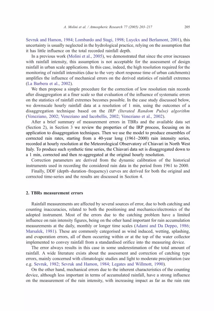
The measurement of rain intensity is traditionally performed by means of tipping-
bucket rain gauges (TBRs), the most popular and widespread type of rain gauge actually
employed worldwide (Fig. 1). These instruments are known to underestimate rainfall at
higher intensities (N100 mm/h) because of the rainwater amount that is lost during the
tipping movement of the buckets. The related biases are known as systematic mechanical
errors and result in the overestimation of rainfall at lower intensities (b50 mm/h) and
underestimation at the higher rain rates (Fankhauser, 1997; La Barbera et al., 2002).
Mechanical errors, although less important in terms of accumulated rainfall, have a
strong influence on the measurement of moderate to high rain intensities, with increasing
impact as far as the rain rate increases.
On the other hand, intense rain-rates are usually characterized by a short duration, so
that any possible correction of the uncertainty connected with mechanical errors strongly
depends on the available resolution in time of the considered time series (Lombardo and
Stagi, 1998).
Though a simple and effective correction technique exists for the bias induced by
systematic mechanical errors, namely dynamic calibration (Marsalek, 1981; Sevruk, 1982;
Fig. 1. The tipping-bucket mechanism (after Marsalek, 1981).
A. Molini et al. / Atmospheric Research 77 (2005) 203–217 205
Sevruk and Hamon, 1984; Lombardo and Stagi, 1998; Luyckx and Berlamont, 2001), this
uncertainty is usually neglected in the hydrological practice, relying on the assumption that
it has little influence on the total recorded rainfall depth.
In a previous work (Molini et al., 2005), we demonstrated that since the error increases
with rainfall intensity, this assumption is not acceptable for the assessment of design
rainfall in urban scale applications. In this case, indeed, the high resolution required for the
monitoring of rainfall intensities (due to the very short response time of urban catchments)
amplifies the influence of mechanical errors on the derived statistics of rainfall extremes
(La Barbera et al., 2002).
We then propose a simple procedure for the correction of low resolution rain records
after disaggregation at a finer scale so that evaluation of the influence of systematic errors
on the statistics of rainfall extremes becomes possible. In the case study discussed below,
we downscale hourly rainfall data at a resolution of 1 min, using the outcomes of a
disaggregation technique based on the IRP (Iterated Random Pulse) algorithm
(Veneziano, 2002; Veneziano and Iacobellis, 2002; Veneziano et al., 2002).
After a brief summary of measurement errors in TBRs and the available data set
(Section 2), in Section 3 we review the properties of the IRP process, focusing on its
application to disaggregation techniques. Then we use the model to produce ensembles of
corrected rain rates, starting from a 40-year long (1961–2000) rain intensity series,
recorded at hourly resolution at the Meteorological Observatory of Chiavari in North West
Italy. To produce such synthetic time series, the Chiavari data set is disaggregated down to
a 1 min, corrected and then re-aggregated at the original hourly resolution.
Correction parameters are derived from the dynamic calibration of the historical
instruments used in recording the considered rain data in the period from 1961 to 2000.
Finally, DDF (depth–duration–frequency) curves are derived for both the original and
corrected time-series and the results are discussed in Section 4.
2. TBRs measurement errors
Rainfall measurements are affected by several sources of error, due to both catching and
counting inaccuracies, related to both the positioning and mechanics/electronics of the
adopted instrument. Most of the errors due to the catching problem have a limited
influence on rain intensity figures, being on the other hand important for rain accumulation
measurements at the daily, monthly or longer time scales (Adami and Da Deppo, 1986;
Marsalek, 1981). These are commonly categorised as wind induced, wetting, splashing,
and evaporation errors, all of them occurring within or at the top of the water collector
implemented to convey rainfall from a standardised orifice into the measuring device.
The error always results in this case in some underestimation of the total amount of
rainfall. A wide literature exists about the assessment and correction of catching type
errors, mainly concerned with climatologic studies and light to moderate precipitation (see
e.g. Sevruk, 1982; Sevruk and Hamon, 1984; Legates and Willmott, 1990).
On the other hand, mechanical errors due to the inherent characteristics of the counting
device, although less important in terms of accumulated rainfall, have a strong influence
on the measurement of the rain intensity, with increasing impact as far as the rain rate
A. Molini et al. / Atmospheric Research 77 (2005) 203–217206
increases. In fact, the measurement of rain intensity, traditionally performed by means of
tipping-bucket rain gauges, is affected by underestimation of rain rates at high intensities
because of the rainwater amount that is lost during the tipping movement of the bucket.
Though this inherent shortcoming can be easily remedied by dynamic calibration (see
later in this section), the usual operational practice in hydro-meteorological services and
instrument manufacturing companies relies on single-point calibration, based on the
assumption that dynamic calibration has little influence on the total recorded rainfall depth
(Fankhauser, 1997).
In two recent papers, the bias introduced by systematic mechanical errors of tipping
bucket rain gauges in the estimation of return periods and other statistics of rainfall
extremes was quantified in very general terms (La Barbera et al., 2002; Molini et al.,
2001), basing on the error figures obtained after laboratory tests over a wide set of
operational rain gauges from the network of the Liguria region in Italy. An equivalent
sample size was also defined as a simple index that can be easily employed by
practitioner engineers to measure the influence of systematic mechanical errors on
common hydrological practice and the derived hydraulic engineering design (La Barbera
et al., 2002).
The bias, estimated in average at about 10–15% for rain rates higher than 200 mm/h, is
strongly specific of the single rain gauge, depending on the manufacturer, the date of
production and the type of wearing (as a function of the existing environmental conditions)
(Becchi, 1970; Marsalek, 1981; Adami and Da Deppo, 1986).
The relevance of such losses, affecting each single tipping of the bucket, increases with
rainfall intensity and is a function of the total time DT requested for the bucket to complete
its rotation. According to Marsalek (1981) the theoretical relationship between the
recorded (Ir) and actual (Ia) intensities as a function of DT is given by:
Ir=Ia ¼ hn= hn þ IaDTð Þ ð1Þ
where hn is the nominal rainfall depth increment per one tip. Note that Ir/Ia=1 only in the
case of DT=0 and that DT is a function of rainfall intensity.
The relationship presented by Marsalek (1981) between DT and Ia shows significant
durations of the bucket movement ranging between 0.3 and 0.6 s for the instruments
analysed. However, the uncertainty involved in the measurement of the time of tipping–
due to the very slow initiation of the bucket rotation–made the comparison of experimental
and theoretical calibration curves hardly appreciable in the author’s work. Sophisticated
measurement of DT allows better success in comparing the experimental calibration curve
with its theoretical expression.
For example, in Luyckx and Berlamont (2001), a theoretical derivation of the
calibration curve is proposed based on a mean value for DT.
However, direct estimation of the calibration curve is far more reliable than its
theoretical derivation as it does not involve sophisticated measurements of very short
intervals in time as a function of varying rain rates. A simple hydraulic apparatus can be
used to this aim, which allows high precision measurements and reliable dynamic
calibration of TBRs (see e.g. Calder and Kidd, 1978; Marsalek, 1981; Niemczynowicz,
1986; Pagliara and Viti, 1994; Lombardo and Stagi, 1998).
A. Molini et al. / Atmospheric Research 77 (2005) 203–217 207
The objective is that of providing the gauge receiver with a constant rain rate at a
number of calibration points in the (Ia, Ir) space. This is achieved by connecting a
constant water level tank with the receiver after interposition of a nozzle with specified
diameter. By modifying the water head over the orifice and the nozzle diameter, constant
flows can be generated at various flow rates as desired (see Humphrey et al., 1997;
Lanza and Stagi, 2002).
Calibration curves reflecting the so-called dynamic calibration of the gauge can be
expressed by means of a power law formulation as:
Ia ¼ a Ibr ð2Þ
where Ia and Ir are again the actual and recorded rain intensities and a, b are calibration
parameters strictly related to the mechanical and wearing characteristics of the considered
TBR. In the practice, Ir is the rainfall intensity recorded during a generic calibration test,
while Ia derives from a more precise measurement device (e.g. a precision balance) placed
in series with the TBR bunder testQ.The two parameters a and b are therefore sufficient to characterise the mechanical
behaviour of the instruments in hand, and to allow correction of the recorded data sets in
order to increase their accuracy.
The associated relative measurement error e can be defined as:
e ¼ Ir � Ia
Ia100 ð3Þ
so that e b0 indicates underestimation rather than overestimation (eN0) of the actual rain
rates.
As an example we report here the results of the dynamic calibration exercise performed
on the three rain gauges that will be used in the following sections to demonstrate the
impact of measuring errors on the estimation of design rainfall. These are the TBR of the
University of Genoa station (available for the period 1990–2002) and the two ones
(manufactured by SILIMET and SIAP) used on successive time spans at the
Meteorological Observatory bAndrea BianchiQ of Chiavari, located about 40 km east of
the town of Genoa along the coastline, and operating since 1883. Concerning the
Meteorological Observatory bAndrea BianchiQ series, a 40-year sub-series is used in this
study (1961–2000). The two series will be hereinafter called the DIAM and the Chiavari
series, respectively. The DIAM data are publicly available online from the University of
Genoa at the following web address: http://www.diam.unige.it/.
In all cases the rain gauge in use was accurately calibrated in the laboratory using the
automatic qualification module for rain intensity measurement instruments developed by
Table 1
Calibration parameters a and b for the three gauges analysed
Station Rain gauge a h
DIAM-University of Genoa CAE (1990–2002) 0.79 1.06
Observatory Andrea Bianchi of Chiavari SIAP (1961–1989) 0.76 1.07
SILIMET (1990–2000) 0.76 1.05
0 50 100 150 200 250 300 3500
50
100
150
200
250
300
350
Recorded Rainfall Intensity Ir [mm/h]
Rai
nfal
l Int
ensi
ty I
[mm
/h]
CAE (DIAm Station)SIAP (Observatory of Chiavari, 1963-1989)SILIMET (Observatory of Chiavari, 1990-2000)
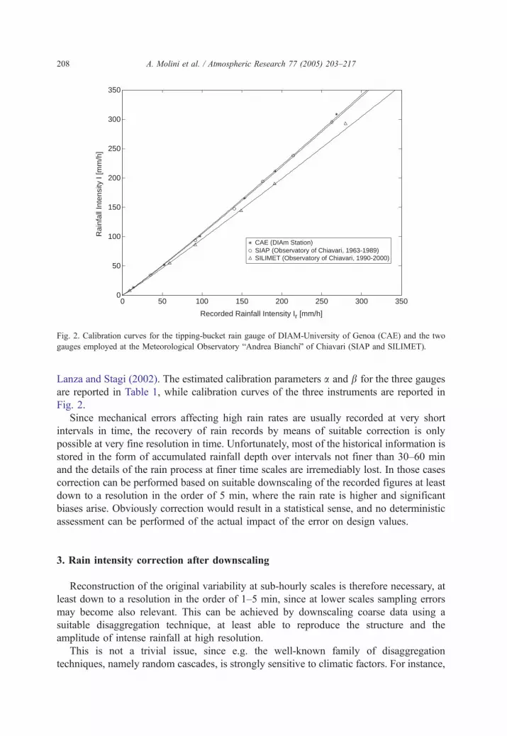
Fig. 2. Calibration curves for the tipping-bucket rain gauge of DIAM-University of Genoa (CAE) and the two
gauges employed at the Meteorological Observatory bAndrea BianchiQ of Chiavari (SIAP and SILIMET).
A. Molini et al. / Atmospheric Research 77 (2005) 203–217208
Lanza and Stagi (2002). The estimated calibration parameters a and b for the three gauges
are reported in Table 1, while calibration curves of the three instruments are reported in
Fig. 2.
Since mechanical errors affecting high rain rates are usually recorded at very short
intervals in time, the recovery of rain records by means of suitable correction is only
possible at very fine resolution in time. Unfortunately, most of the historical information is
stored in the form of accumulated rainfall depth over intervals not finer than 30–60 min
and the details of the rain process at finer time scales are irremediably lost. In those cases
correction can be performed based on suitable downscaling of the recorded figures at least
down to a resolution in the order of 5 min, where the rain rate is higher and significant
biases arise. Obviously correction would result in a statistical sense, and no deterministic
assessment can be performed of the actual impact of the error on design values.
3. Rain intensity correction after downscaling
Reconstruction of the original variability at sub-hourly scales is therefore necessary, at
least down to a resolution in the order of 1–5 min, since at lower scales sampling errors
may become also relevant. This can be achieved by downscaling coarse data using a
suitable disaggregation technique, at least able to reproduce the structure and the
amplitude of intense rainfall at high resolution.
This is not a trivial issue, since e.g. the well-known family of disaggregation
techniques, namely random cascades, is strongly sensitive to climatic factors. For instance,
A. Molini et al. / Atmospheric Research 77 (2005) 203–217 209
disaggregation schemes basing on the classical multiplicative random cascade can produce
unrealistic rain intensities when calibrated on mid-latitudes data (Guntner et al., 2001;
Mouhous et al., 2001), then making statistical correction less effective.
In this section we apply the correction procedure to the coarse resolution rain intensity
data of the Chiavari series after downscaling based on the IRP (Iterated Random Pulse)
algorithm. After a brief review of the model, the Chiavari data set, is disaggregated at 1-
min resolution, corrected using the parameters obtained after dynamic calibration of the
involved TBRs and therefore re-aggregated at hourly resolution. The calibration curves of
the two TBRs used at the Chiavari station in the period 1961–2000 are reported in Fig. 2.
The basic parameters of the model, the co-dimension and the contraction factor, have been
respectively obtained from the literature (Veneziano and Iacobellis, 2002) and after
accurate calibration of the model on the data of the DIAm series.
The procedure has been repeated 1000 times, so that an ensemble of as much 40
year2long synthetic series was obtained. Traditional DDF curves and extreme statistics
have been calculated in order to assess the influence of the applied correction. To infer
DDF curves, independence was assumed for annual maxima and the related parameters
were derived after fitting an extreme value distribution (EV1 or Gumbel).
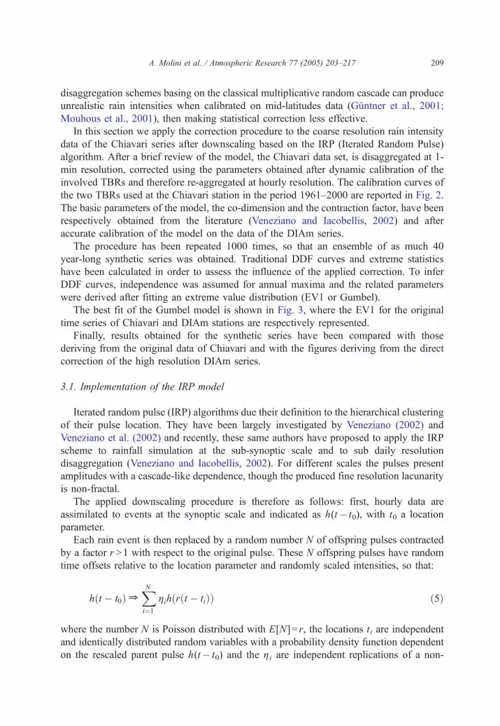
The best fit of the Gumbel model is shown in Fig. 3, where the EV1 for the original
time series of Chiavari and DIAm stations are respectively represented.
Finally, results obtained for the synthetic series have been compared with those
deriving from the original data of Chiavari and with the figures deriving from the direct
correction of the high resolution DIAm series.
3.1. Implementation of the IRP model
Iterated random pulse (IRP) algorithms due their definition to the hierarchical clustering
of their pulse location. They have been largely investigated by Veneziano (2002) and
Veneziano et al. (2002) and recently, these same authors have proposed to apply the IRP
scheme to rainfall simulation at the sub-synoptic scale and to sub daily resolution
disaggregation (Veneziano and Iacobellis, 2002). For different scales the pulses present
amplitudes with a cascade-like dependence, though the produced fine resolution lacunarity
is non-fractal.
The applied downscaling procedure is therefore as follows: first, hourly data are
assimilated to events at the synoptic scale and indicated as h(t� t0), with t0 a location
parameter.
Each rain event is then replaced by a random number N of offspring pulses contracted
by a factor r N1 with respect to the original pulse. These N offspring pulses have random
time offsets relative to the location parameter and randomly scaled intensities, so that:
h t � t0ð Þ ZXN
i¼1
gih r t � tið Þð Þ ð5Þ
where the number N is Poisson distributed with E[N]= r, the locations ti are independent
and identically distributed random variables with a probability density function dependent
on the rescaled parent pulse h(t� t0) and the gi are independent replications of a non-
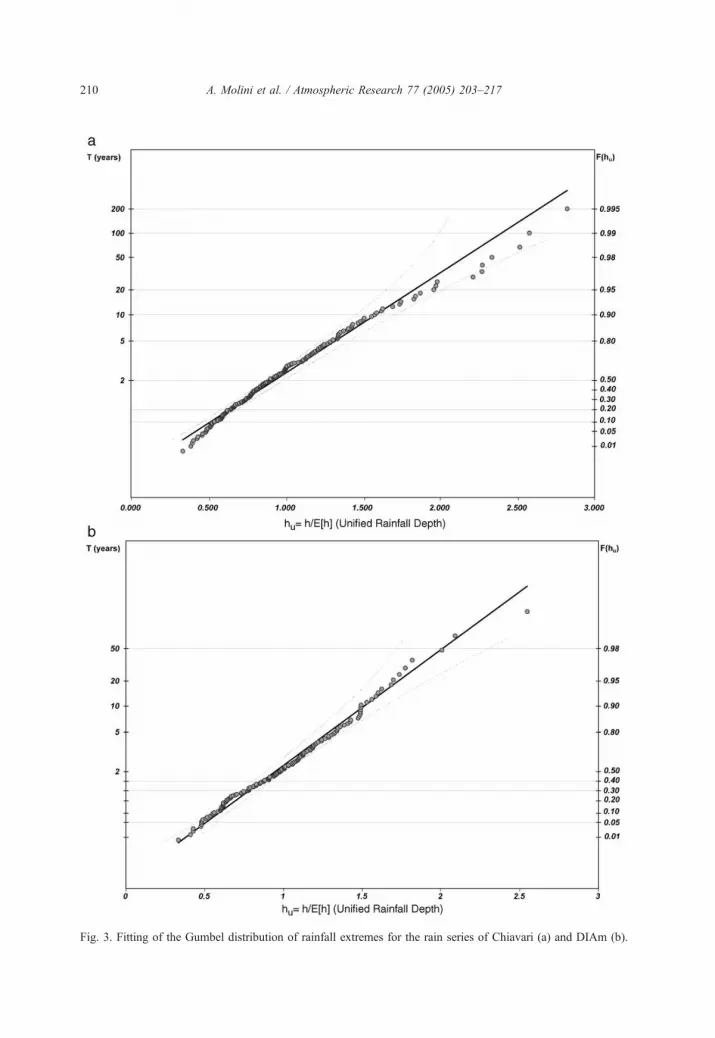
Fig. 3. Fitting of the Gumbel distribution of rainfall extremes for the rain series of Chiavari (a) and DIAm (b).
A. Molini et al. / Atmospheric Research 77 (2005) 203–217210
Jan Feb Mar Apr May Jun Jul Aug Sep Oct Nov Dec0
2
4
6
8
10
12
Meteorological Observatory of Chiavari, Genova – Simulated rainfall depth cumulated on 1 minute (mm): year=1995
month
Rai
nfal
l dep
th (
mm
) –
Agg
rega
tion=
1 m
inut
e
Jan Feb Mar Apr May Jun Jul Aug Sep Oct Nov Dec0
2
4
6
8
10
12
14
Dept. of Environmental Engineering, University of Genova – Rainfall depth cumulated on 1 minute (mm): year=1995
µ= 0.0032 mmσ2= 0.0019 mm2
rainy periods= 1.07 %lost data= 3.56 %
µrr>0= 0.286 mm
σrr>0= 0.095 mm2
max on 1 minute= 9.4 mm
month
Rai
nfal
l dep
th (
mm
) –
Agg
rega
tion=
1 m
inut
e
–––
–––
µ= 0.0018 mmσ2= 0.0010 mm2
rainy periods= 0.68 %
µrr>0= 0.269 mm
σrr>0= 0.077 mm2
max on 1 minute= 7.6 mm
–––
–––
a
b
2
2
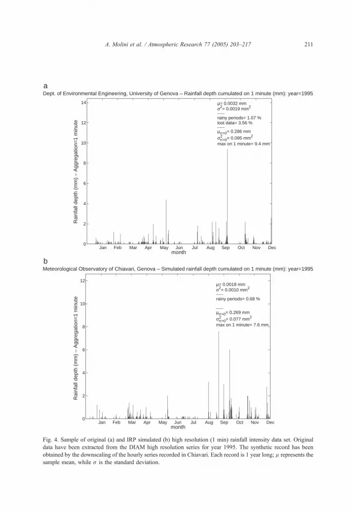
Fig. 4. Sample of original (a) and IRP simulated (b) high resolution (1 min) rainfall intensity data set. Original
data have been extracted from the DIAM high resolution series for year 1995. The synthetic record has been
obtained by the downscaling of the hourly series recorded in Chiavari. Each record is 1 year long; l represents the
sample mean, while r is the standard deviation.
A. Molini et al. / Atmospheric Research 77 (2005) 203–217 211
0 3 6 9 12 15 18 21 2430
40
50
60
70
80
90
100
duration (hours)
rain
fall
dept
h (m
m)
T=2 years
0 3 6 9 12 15 18 21 2460
70
80
90
100
110
120
130
140
150
160
170
duration (hours)
rain
fall
dept
h (m
m)
T=10 years
0 3 6 9 12 15 18 21 2460
80
100
120
140
160
180
200
duration (hours)
rain
fall
dept
h (m
m)
T=20 years
0 3 6 9 12 15 18 21 2480
100
120
140
160
180
200
220
240
duration (hours)
rain
fall
dept
h (m
m)
T=50 years
0 3 6 9 12 15 18 21 2480
100
120
140
160
180
200
220
240
260
duration (hours)
rain
fall
dept
h (m
m)
T=100 years
0 3 6 9 12 15 18 21 24100
120
140
160
180
200
220
240
260
280
duration (hours)
rain
fall
dept
h (m
m)
T=200 years
a b
c d
e f
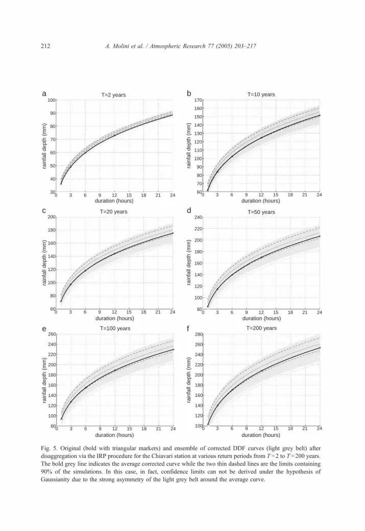
Fig. 5. Original (bold with triangular markers) and ensemble of corrected DDF curves (light grey belt) after
disaggregation via the IRP procedure for the Chiavari station at various return periods from T=2 to T =200 years.
The bold grey line indicates the average corrected curve while the two thin dashed lines are the limits containing
90% of the simulations. In this case, in fact, confidence limits can not be derived under the hypothesis of
Gaussianity due to the strong asymmetry of the light grey belt around the average curve.
A. Molini et al. / Atmospheric Research 77 (2005) 203–217212
A. Molini et al. / Atmospheric Research 77 (2005) 203–217 213
negative random variable g with mean value 1. The process is then iteratively reproduced
at all the successive disaggregation steps.
Moreover, according to Veneziano and Iacobellis (2002), the distribution of g was
assumed lognormal, so that only two parameters have to be estimated: the contraction
factor r (here assumed equal to 4) and the co-dimension C1=0.5 logr(Etg2b) (here assumed
equal to 0.1, i.e. the same value estimated by Veneziano and Iacobellis, 2002 on the long
duration time series of Florence).
The value of the contraction factor r has been obtained from the calibration of the
model on the DIAm high resolution series. In Fig. 4 a qualitative comparison between the
year 1995 sub-series from DIAM and 1 year of IRP simulated high resolution (1 min)
rainfall depths, is reported.
The ensemble of DDF curves (for 1000 simulations) obtained after suitable correction
and re-aggregation of the IRP disaggregated data is reported in Fig. 5 for different return
periods T.
The original data are represented by the bold line with triangular markers, while the
light grey belt is the ensemble of corrected DDF curves after disaggregation using the IRP
procedure. The bold grey line indicates the average corrected curve while the two thin
dashed lines are the limits containing 90% of the simulations.
4. Discussion of the results
The accuracy of the proposed correction procedure of historical rainfall time series is
obviously dependent on the reliability of the adopted disaggregation technique. It is
therefore evident that in case the downscaling procedure should produce unrealistic
rainfall intensities at finer scales, the validity of the corrected figures actually breaks
down. In a previous work (Molini et al., 2005), we proposed correction of historical
rainfall data, based on the canonical random cascade algorithm for rainfall downscaling.
That model generally overestimates high rainfall intensities at fine resolution, due to its
tendency to concentrate extreme intensities on very short time durations. This fact
directly derives from the parameter estimation procedure, where the weights deriving
from the down-scaling of low to medium events–i.e. the most frequent occurrences–
assume a more relevant role than the generators coming from the disaggregation of
extreme events (marginally probable) presenting a more complex correlation structure.
This model is therefore more suitable for arid zones, where convective events
constitutes the 90% of total events, rather than for the considered mid-latitude regions,
characterized by both convective and frontal events, with very different characteristics
(Guntner et al., 2001). We then concluded that comparison of different algorithms
would be desirable although it is quite reasonable that the resulting correction on the
statistical parameters will be basically determined by the imposed variance of the inner
scale process.
This observation is confirmed by the results obtained here from the IRP based
disaggregation model where, even if the substantial underestimation of return periods and
extreme statistics is still evident, the influence of measurement errors seems to be less
pronounced.
1
1.02
1.04
1.06
1.08
1.1
01E+00 10E+00 01E+02
duration (hours)
h cor
rect
ed/h
orig
inal
T=2
T=10
T=20
T=50
T=100
T=200
Return PeriodT (years)
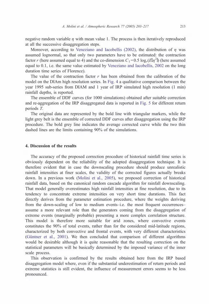
Fig. 6. Synthetic representation of the bgainQ obtained after correction of the high resolution realisations obtained
from downscaling hourly records from the Chiavari station using IRP.
A. Molini et al. / Atmospheric Research 77 (2005) 203–217214
At the same time, the ensemble average curve for the IRP simulated data appears
shifted towards the zone of the curves that is more affected by correction, producing a sort
of low correction tail below the curve of the original data. This fact, combined with a
10-2 10-1 100 101 1021
1.02
1.04
1.06
1.08
1.1
1.12
1.14
1.16
1.18
duration (hours)
h cor
rect
ed/h
orig
inal
Return Period
T (years)
T=2
T=10
T=20
T=50
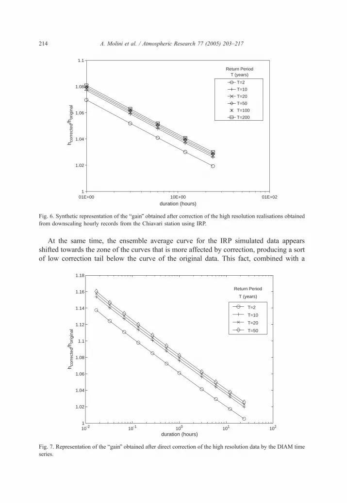
Fig. 7. Representation of the bgainQ obtained after direct correction of the high resolution data by the DIAM time
series.
A. Molini et al. / Atmospheric Research 77 (2005) 203–217 215
wider dispersion of IRP based series, is probably due to the skill of IRP processes in better
representing strongly correlated events (that are also the ones with higher volumes) and, at
the same time, in preserving the variance of the process at fine scales (low tail).
The assessment of the relative error on maximum depths as a function of duration in time,
is represented for the IRP synthetic data in Fig. 6. Here the deviation of corrected data from
the original ones is represented in the form of a bgainQ varying with duration and seems to
suggest the presence of a strong underestimation of total maximum volumes for the lowest
traditionally considered durations (the most relevant in urban hydrology applications).
In Fig. 7, the bgainQ is reported as a function of duration, for the 1 min DIAM series
after direct correction using the parameters in Table 1 has been performed. The corrected
0.9
1
1.1
1.2
1.3
1.4
1.5
1.6
1.7
1.8
1.9
1 10 100 1000T (years)
Tor
igin
al/T
corr
ecte
dT
orig
inal
/Tco
rrec
ted
IRP SimulatedDIAM high resolution series
duration=1 hour
0.9
1
1.1
1.2
1.3
1.4
1.5
1.6
1.7
1.8
1.9
1 10 100 1000 T (years)
IRP SimulatedDiam high resolution series
duration=24 hour
a
b
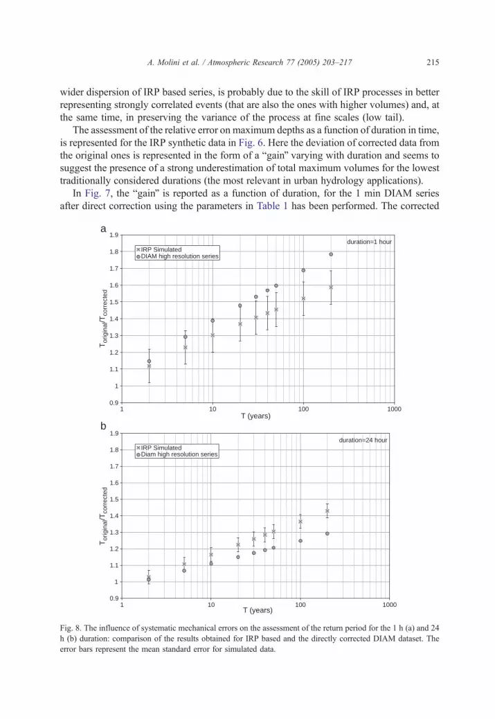
Fig. 8. The influence of systematic mechanical errors on the assessment of the return period for the 1 h (a) and 24
h (b) duration: comparison of the results obtained for IRP based and the directly corrected DIAM dataset. The
error bars represent the mean standard error for simulated data.
A. Molini et al. / Atmospheric Research 77 (2005) 203–217216
DIAM series constitute an important reference for the performance of the correction
procedure.
Again, the underestimation of maximum depths in IRP synthetic data for T=50 years
and 1 h duration is about 8–9%, denoting a good agreement with directly corrected data
(8%).
Finally, in Fig. 8(a) and (b) the influence of systematic mechanical errors on the
assessment of the return period for the 1 h and 24 h durations is represented for the IRP
and directly corrected data. The error bars represent the mean standard error for simulated
data.
In particular, for directly corrected data, the induced bias can be quantified as an error
of 80% on the assessment of the return period of design rainfall for duration 1 h, when the
return period is in the order of 200 years, against the 60% of IRP simulated records.
Obviously, in analysing these results the fact that the two series (Chiavari Observatory
and DIAM) were recorded at different locations must be properly taken into account.
Acknowledgements
The authors express their sincere thanks to Roberto Picasso, Director of the
Meteorological Observatory bAndrea BianchiQ of Chiavari, for his kindness in providing
the rain data collected over the period 1961–2000 and to the whole group of volunteers at
the observatory, particularly to Alberto Ansaloni, for the precious contribution provided in
the reconstruction of the history of the observations and of the various rain gauge
instruments employed.
We also wish to thank Vito Iacobellis for his precious suggestions about the IRP
algorithm and its application to rainfall disaggregation.
References
Adami, A., Da Deppo, L., 1986. On the systematic errors of tipping bucket recording rain gauges. Proc. Int.
Workshop on the Correction of Precipitation Measurements, Zurich, Switzerland, 1–3 April 1985.
Becchi, I., 1970. On the possibility of improving rain measurements: calibration of tipping-bucket rain gauges.
(in Italian). Tech. Rep. For CNR grant no. 69.01919. University of Genoa, p. 11.
Calder, I.R., Kidd, C.H.R., 1978. A note on the dynamic calibration of tipping-bucket gauges. J. Hydrol. 39,
383–386.
Fankhauser, R., 1997. Measurement properties of tipping bucket rain gauges and their influence on urban runoff
simulation. Water Sci. Technol. 36 (8–9), 7–12.
Guntner, A., Olsson, J., Calver, A., Gannon, B., 2001. Cascade-based disaggregation of continuous rainfall time
series: the influence of climate. Hydrol. Earth Syst. Sci. 5, 145–164.
Humphrey, M.D., Istok, J.D., Lee, J.Y., Hevesi, J.A., Flint, A.L., 1997. A new method for automated calibration
of tipping-bucket rain gauges. J. Atmos. Ocean. Technol. 14, 1513–1519.
Keifer, C.J., Chu, H.H., 1957. Synthetic storm pattern for drainage design. J. Hydraul. Div., Am. Soc. Civ. Eng.
83 (HY4), 1–25.
La Barbera, P., Lanza, L.G., Stagi, L., 2002. Tipping bucket mechanical errors and their influence on rainfall
statistics and extremes. Water Sci. Technol. 45 (2), 1–9.
Lanza, L. and Stagi, L., 2002. Quality standards for rain intensity measurements. WMO Commission on
Instruments and Observing Methods-Rep. N8 75 - WMO/TD-No.1123, P2(4). Published on CD-ROM.
A. Molini et al. / Atmospheric Research 77 (2005) 203–217 217
Legates, D.R., Willmott, C.J., 1990. Mean seasonal and spatial variability in gauge-corrected, global precipitation.
Int. J. Climatol. 10, 111–127.
Lombardo, F., Stagi, L., 1998. Testing and dynamic calibration of rain gauges aimed at the assessment of
errors for intense rainfall (in Italian). Proc. XXVI Conf. On Hydraulics and Hydraulic Structures, CUECM
Ed., Catania, pp. 85–96.
Luyckx, G., Berlamont, J., 1981. Simplified method to correct rainfall measurements from tipping bucket rain
gauges. Proc. Of the World Water and Environmental Resources (EWRI) Congress-Urban Drainage
Modelling (UDM) Symposium, Orlando, 20–24 May 2001.
Marsalek, J., 1981. Calibration of the tipping bucket raingauge. J. Hydrol. 53, 343–354.
Molini, A., La Barbera, P., Lanza, L.G., Stagi, L., 2001. Rainfall intermittency and the sampling error of tipping-
bucket rain gauges. Phys. Chem. Earth 26 (10–12), 737–742.
Molini, A., La Barbera, P., Lanza, L.G., Stagi, L., 2005. The impact of TBRs measurement errors on design
rainfall for urban-scale applications. Hydrol. Process. 19, 1073–1088.
Mouhous, N., Gaume, E., Andrieu, H., 2001. Influence of the Highest Values on the Choice of Log-Poisson
Random Cascade Model Parameters. Phys. Chem. Earth, B 26 (9), 701–704.
Niemczynowicz, J., 1986. The dynamic calibration of tipping-bucket raingauges. Nord. Hydrol. 17, 203–214.
Pagliara, S., Viti, C., 1994. Dynamic calibration of a tipping-bucket rain gauge sensor (in Italian). Boll. Geofis. 2,
63–69.
Sevruk, B., 1982. Methods of correction for systematic error in point precipitation measurement for operational
use. WMO Rep. N8 589, Operational Hydrology Report, vol. 21, p. 91.
Sevruk, B., Hamon, W.R., 1984. International comparison of national precipitation gauges with a reference pit
gauge. Instruments and Observing Methods Report, vol. 17. WMO, p. 86.
Veneziano, D., 2002. Iterated random pulse processes and their spectral properties. Fractals 10 (1), 1–11.
Veneziano, D., Iacobellis, V., 2002. Multiscaling pulse representation of temporal rainfall. Water Resour. Res.
38 (8).
Veneziano, D., Furcolo, P.L., Iacobellis, V., 2002. Multifractality of iterated pulse processes with pulse amplitudes
generated by a random cascade. Fractals 10 (2), 209–222.


