Scaling behavior of heavy fermion metalsV.R. Shaginyan a,b,∗, M.Ya. Amusia c,d, A.Z. Msezane b, K.G. Popov ea Petersburg Nuclear Physics Institute, RAS, Gatchina, 188300, Russiab CTSPS, Clark Atlanta University, Atlanta, GA 30314, USAc Racah Institute of Physics, Hebrew University, Jerusalem 91904, Israeld Ioffe Physical Technical Institute, RAS, St. Petersburg 194021, Russiae Komi Science Center, Ural Division, RAS, 3a, Chernova str. Syktyvkar, 167982, Russia
a r t i c l e i n f o
Article history:Accepted 4 March 2010Available online 24 March 2010editor: D.L. Mills
Strongly correlated Fermi systems are fundamental systems in physics that are best studiedexperimentally,which until very recently have lacked theoretical explanations. This reviewdiscusses the construction of a theory and the analysis of phenomena occurring in stronglycorrelated Fermi systems such as heavy-fermion (HF) metals and two-dimensional (2D)Fermi systems. It is shown that the basic properties and the scaling behavior of HFmetals can be described within the framework of a fermion condensation quantum phasetransition (FCQPT) and an extended quasiparticle paradigm that allow us to explain thenon-Fermi liquid behavior observed in strongly correlated Fermi systems. In contrast tothe Landau paradigm stating that the quasiparticle effectivemass is a constant, the effectivemass of new quasiparticles strongly depends on temperature, magnetic field, pressure, andother parameters. Having analyzed the collected facts on strongly correlated Fermi systemswith quite a different microscopic nature, we find these to exhibit the same non-Fermiliquid behavior at FCQPT. We show both analytically and using arguments based entirelyon the experimental grounds that the data collected on very different strongly correlatedFermi systems have a universal scaling behavior, and materials with strongly correlatedfermions can unexpectedly be uniform in their diversity. Our analysis of strongly correlatedsystems such as HF metals and 2D Fermi systems is in the context of salient experimentalresults. Our calculations of the non-Fermi liquid behavior, the scales and thermodynamic,relaxation and transport properties are in good agreement with experimental facts.
1. Introduction............................................................................................................................................................................................. 321.1. Quantum phase transitions and the non-Fermi liquid behavior of correlated Fermi systems.............................................. 331.2. Limits and goals of the review ................................................................................................................................................... 35
2. Landau theory of Fermi liquids .............................................................................................................................................................. 363. Equation for the effective mass and the scaling behavior .................................................................................................................... 374. Fermion condensation quantum phase transition................................................................................................................................ 39
4.1. The order parameter of FCQPT................................................................................................................................................... 404.2. Quantum protectorate related to FCQPT ................................................................................................................................... 414.3. The influence of FCQPT at finite temperatures ......................................................................................................................... 424.4. Phase diagram of Fermi system with FCQPT............................................................................................................................. 43
5. The superconducting state with FC........................................................................................................................................................ 445.1. The superconducting state at T = 0.......................................................................................................................................... 445.2. Green’s function of the superconducting state with FC at T = 0 ............................................................................................ 455.3. The superconducting state at finite temperatures ................................................................................................................... 465.4. Bogoliubov quasiparticles .......................................................................................................................................................... 465.5. The pseudogap ............................................................................................................................................................................ 475.6. Dependence of the critical temperature Tc of the superconducting phase transition on doping ......................................... 495.7. The gap and heat capacity near Tc ............................................................................................................................................. 49
6. The dispersion law and lineshape of single-particle excitations ......................................................................................................... 507. Electron liquid with FC in magnetic fields............................................................................................................................................. 52
7.1. Phase diagram of electron liquid in magnetic field .................................................................................................................. 527.2. Dependence of effective mass on magnetic fields in HF metals and high-Tc superconductors ............................................ 54
7.2.1. Common QCP in the high-Tc Tl2Ba2CuO6+x and the HF metal YbRh2Si2 ................................................................. 558. Appearance of FCQPT in Fermi systems................................................................................................................................................. 569. A highly correlated Fermi liquid in HF metals ...................................................................................................................................... 58
9.1. Dependence of the effective massM∗ on magnetic field......................................................................................................... 589.2. Dependence of the effective massM∗ on temperature and the damping of quasiparticles.................................................. 599.3. Scaling behavior of the effective mass ...................................................................................................................................... 61
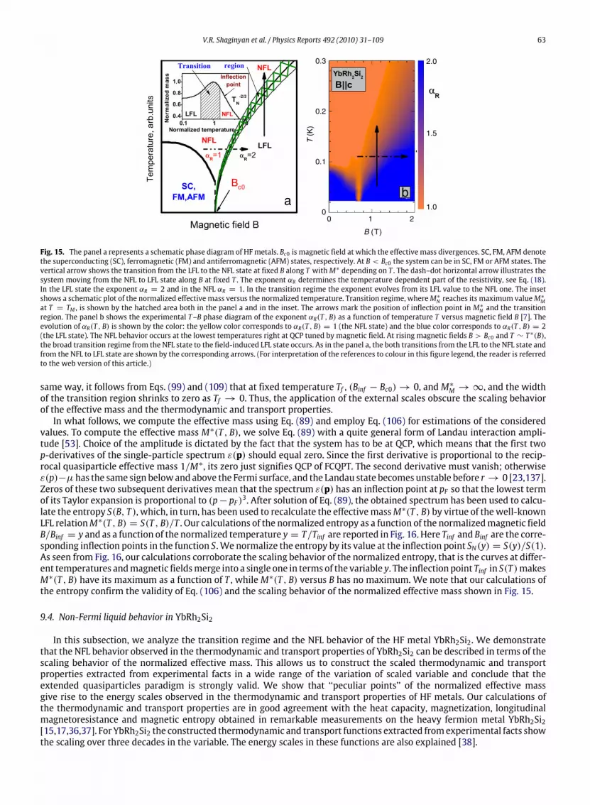
9.3.1. Schematic phase diagram of HF metal ....................................................................................................................... 629.4. Non-Fermi liquid behavior in YbRh2Si2 .................................................................................................................................... 63
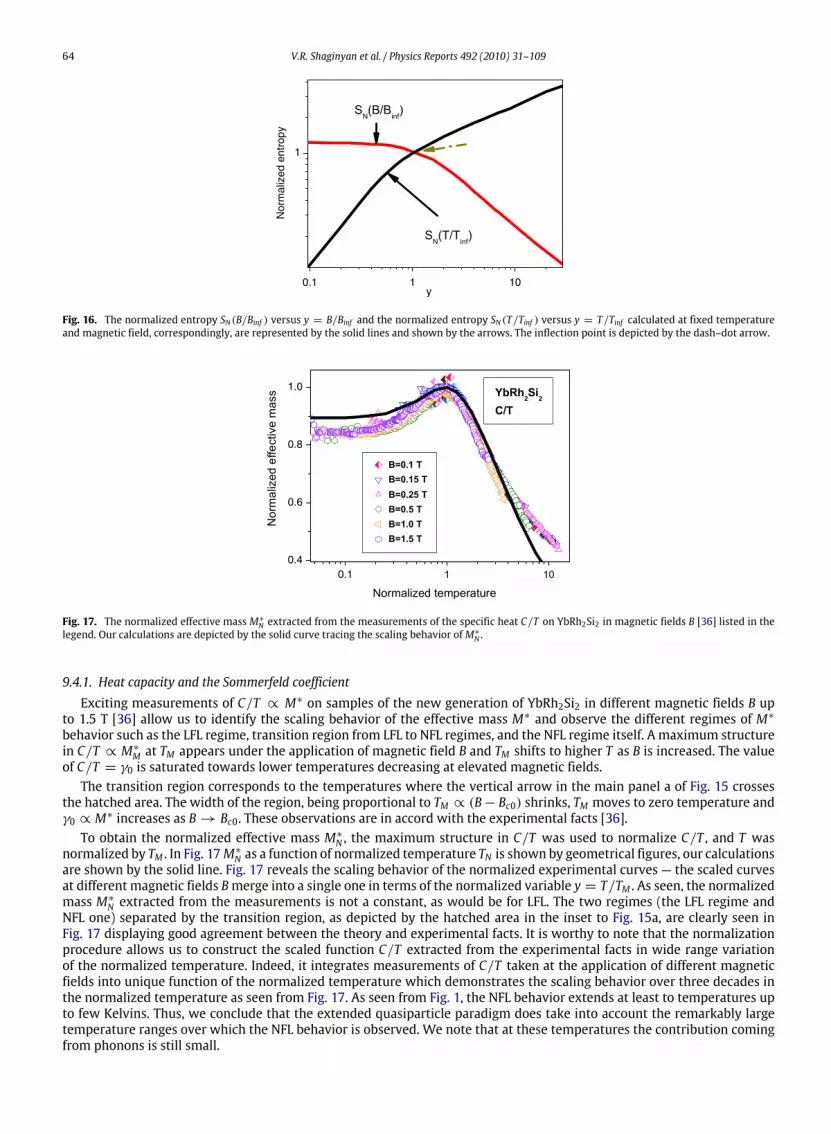
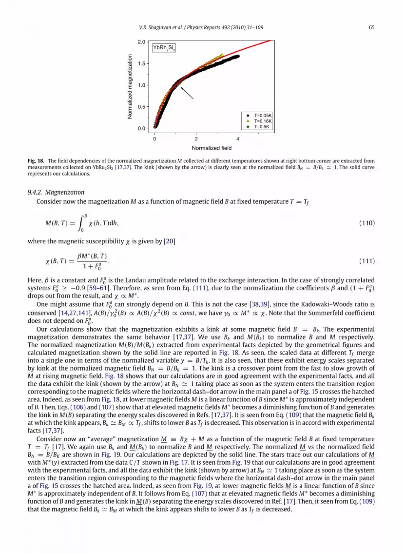
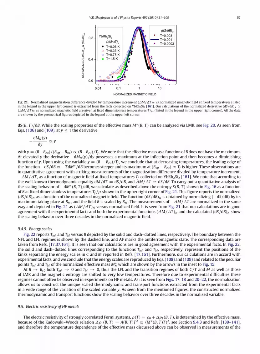
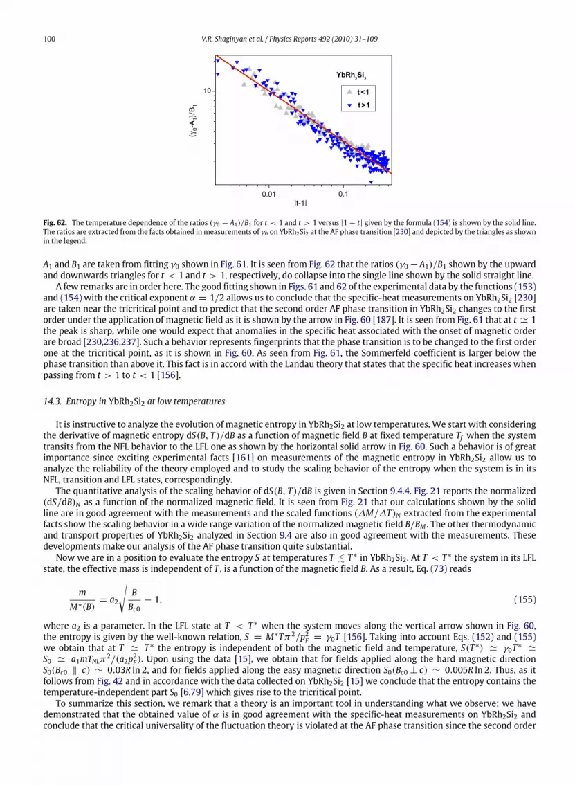
9.4.1. Heat capacity and the Sommerfeld coefficient .......................................................................................................... 649.4.2. Magnetization .............................................................................................................................................................. 659.4.3. Longitudinal magnetoresistance ................................................................................................................................ 669.4.4. Magnetic entropy......................................................................................................................................................... 669.4.5. Energy scales ................................................................................................................................................................ 67
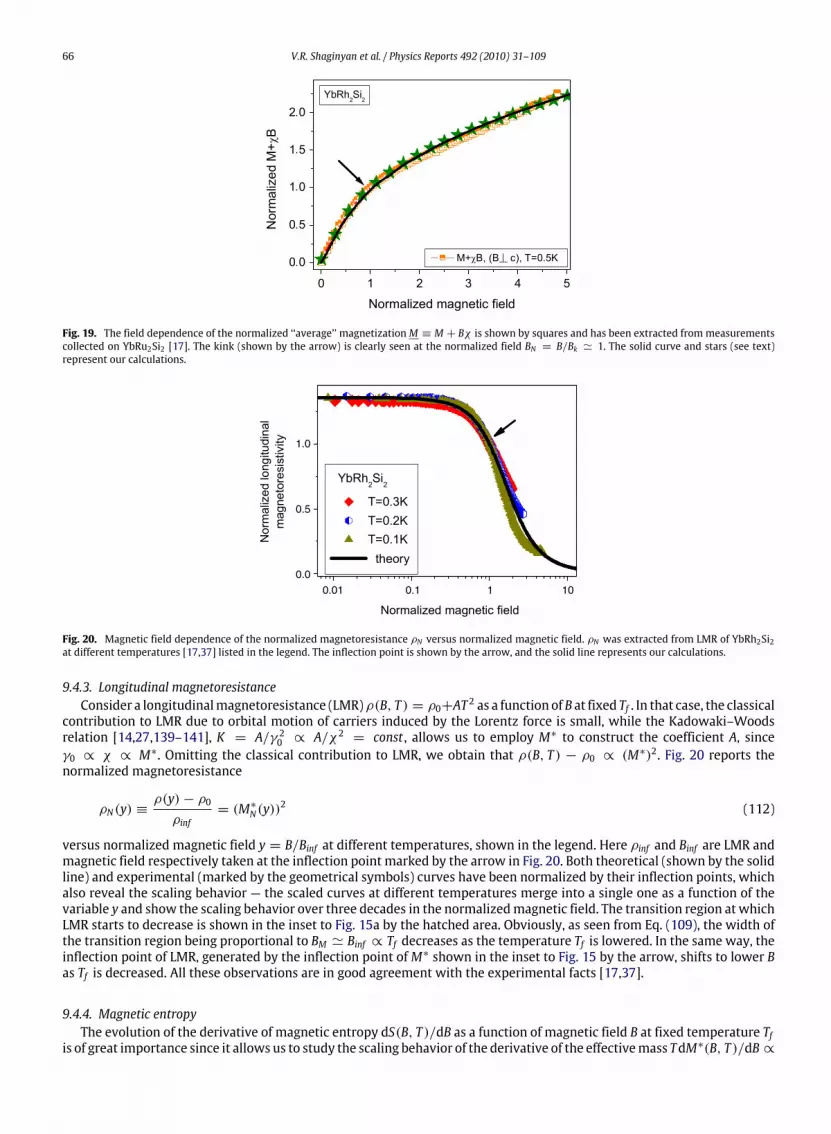
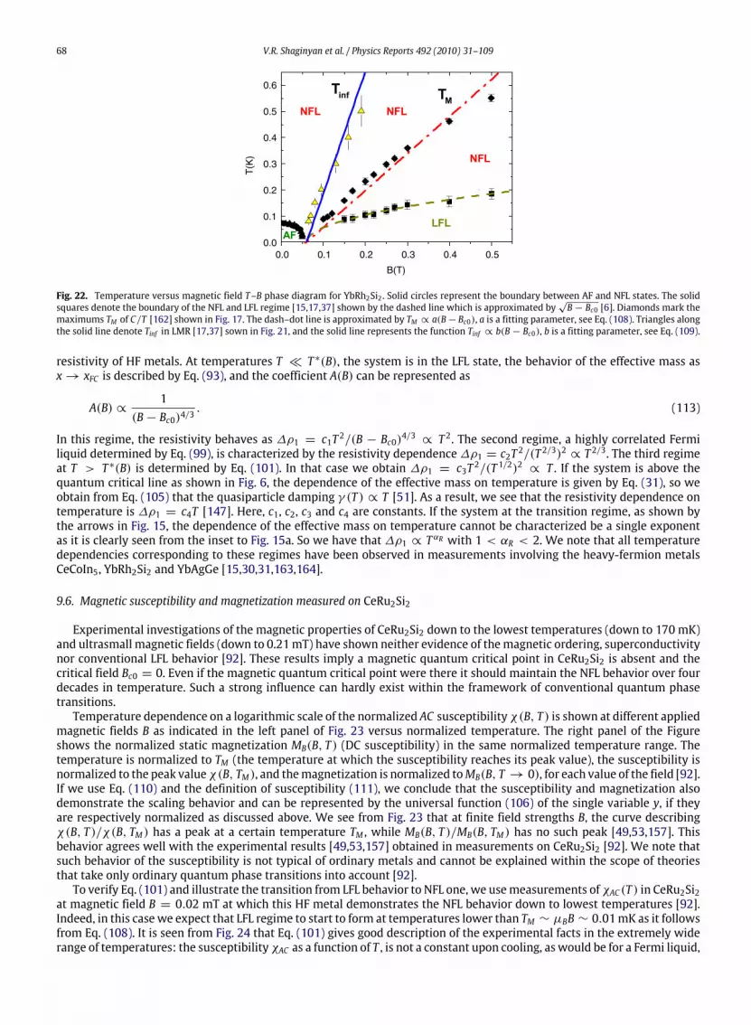
9.5. Electric resistivity of HF metals ................................................................................................................................................. 679.6. Magnetic susceptibility and magnetization measured on CeRu2Si2 ....................................................................................... 689.7. Transverse magnetoresistance in the HF metal CeCoIn5 ......................................................................................................... 699.8. Magnetic-field-induced reentrance of Fermi-liquid behavior and spin-lattice relaxation rates in YbCu5−xAux ................. 719.9. Relationships between critical magnetic fields Bc0 and Bc2 in HF metals and high-Tc superconductors ............................. 749.10. Scaling behavior of the HF CePd1−xRhx ferromagnet ............................................................................................................... 76
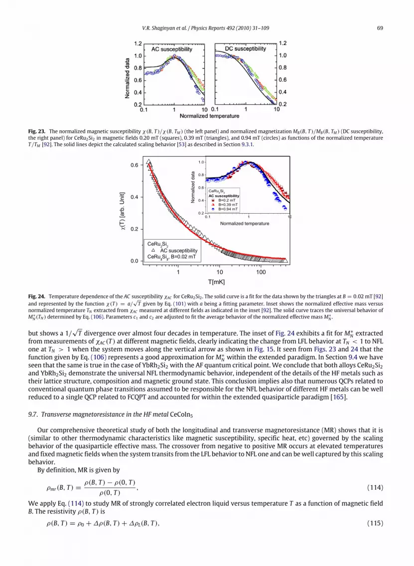
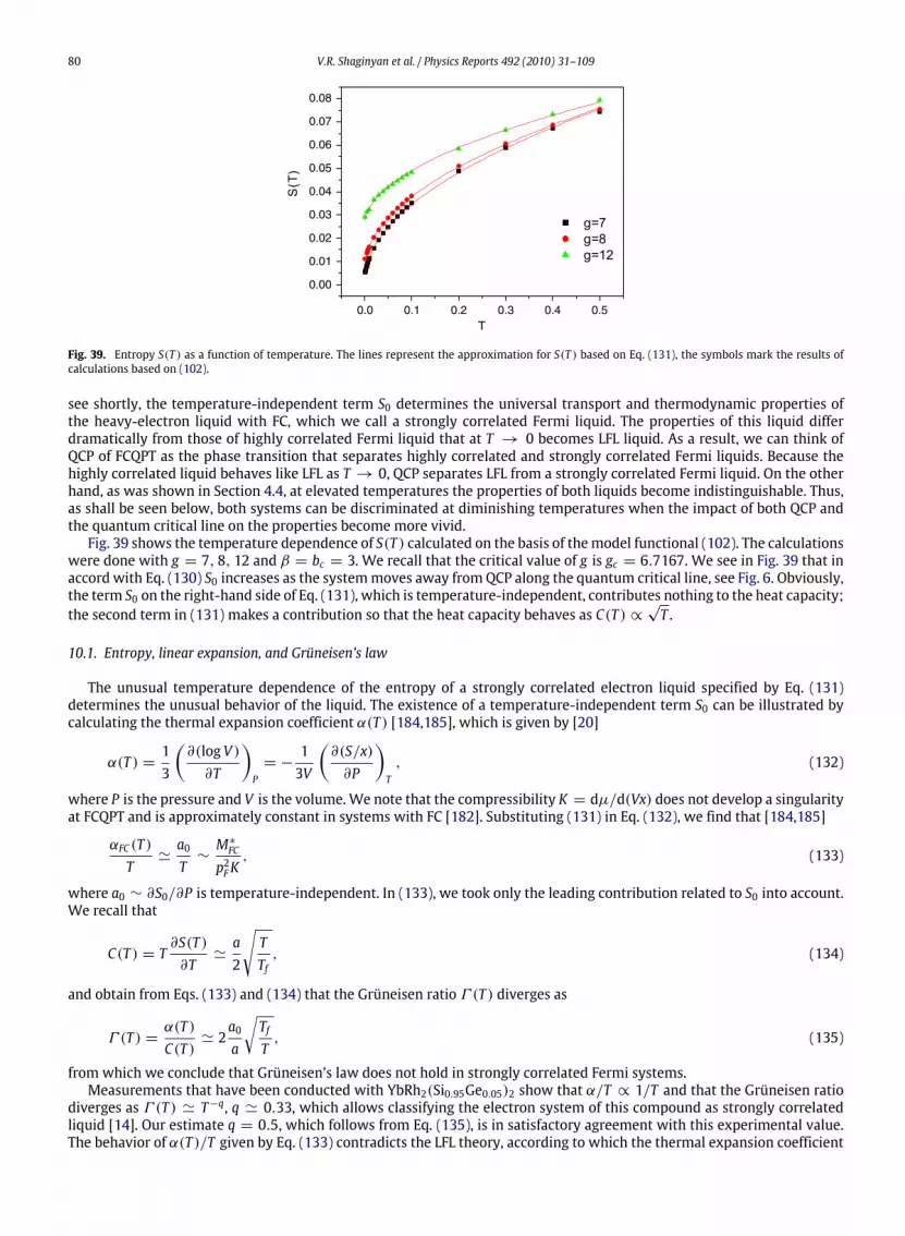
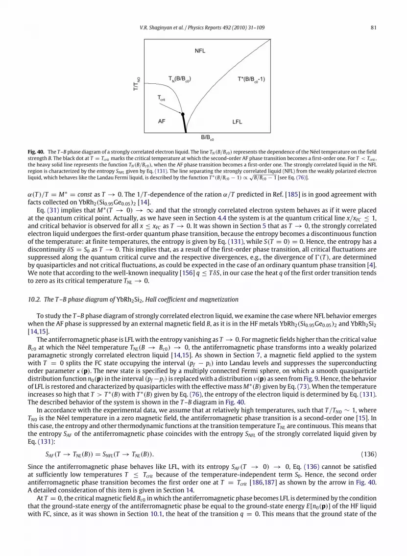
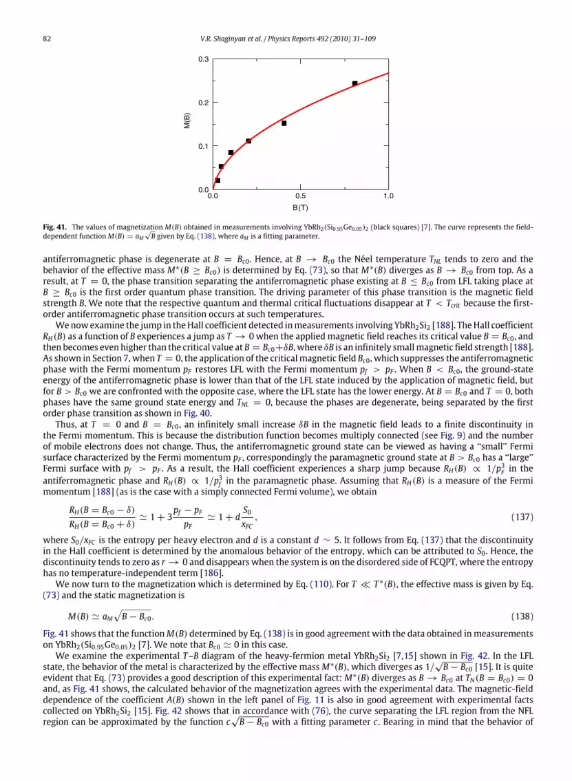
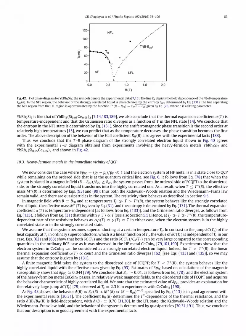
10. Metals with a strongly correlated electron liquid................................................................................................................................. 7910.1. Entropy, linear expansion, and Grüneisen’s law....................................................................................................................... 8010.2. The T–B phase diagram of YbRh2Si2, Hall coefficient and magnetization .............................................................................. 8110.3. Heavy-fermion metals in the immediate vicinity of QCP ........................................................................................................ 83
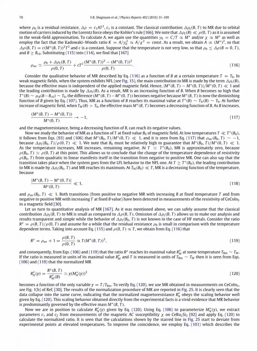
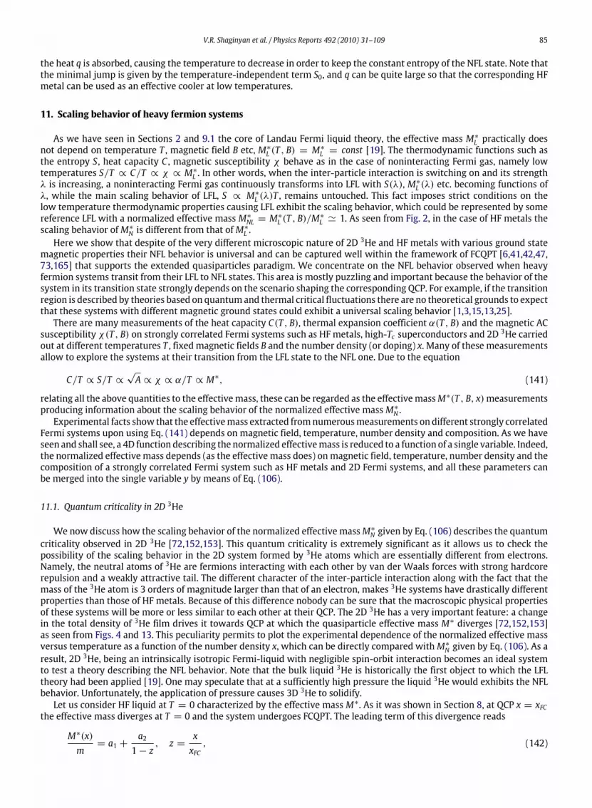
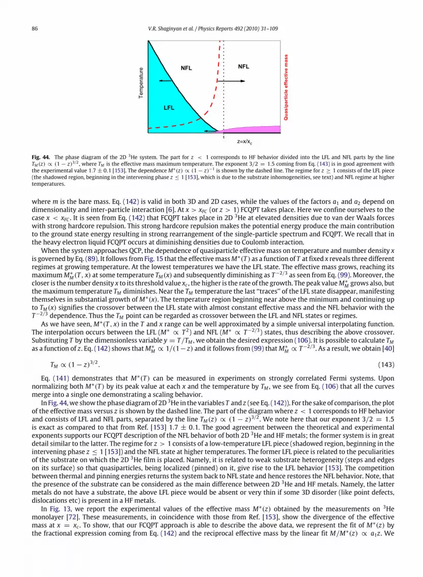
11. Scaling behavior of heavy fermion systems .......................................................................................................................................... 8511.1. Quantum criticality in 2D 3He ................................................................................................................................................... 8511.2. Kinks in the thermodynamic functions ..................................................................................................................................... 8811.3. Heavy-fermion metals at metamagnetic phase transitions..................................................................................................... 89
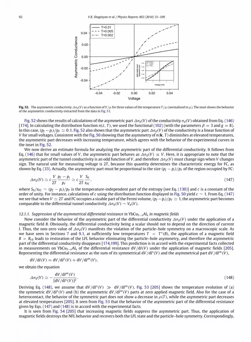
12. Asymmetric conductivity in HF metals and high-Tc superconductors................................................................................................ 9012.1. Normal state................................................................................................................................................................................ 90
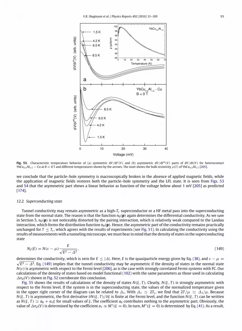
12.1.1. Suppression of the asymmetrical differential resistance in YbCu5−xAlx in magnetic fields ................................... 9212.2. Superconducting state ................................................................................................................................................................ 93
13. Violation of the Wiedemann–Franz law in HF metals .......................................................................................................................... 9614. The impact of FCQPT on ordinary continuous phase transitions in HF metals ................................................................................... 97
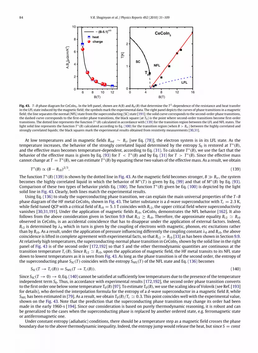
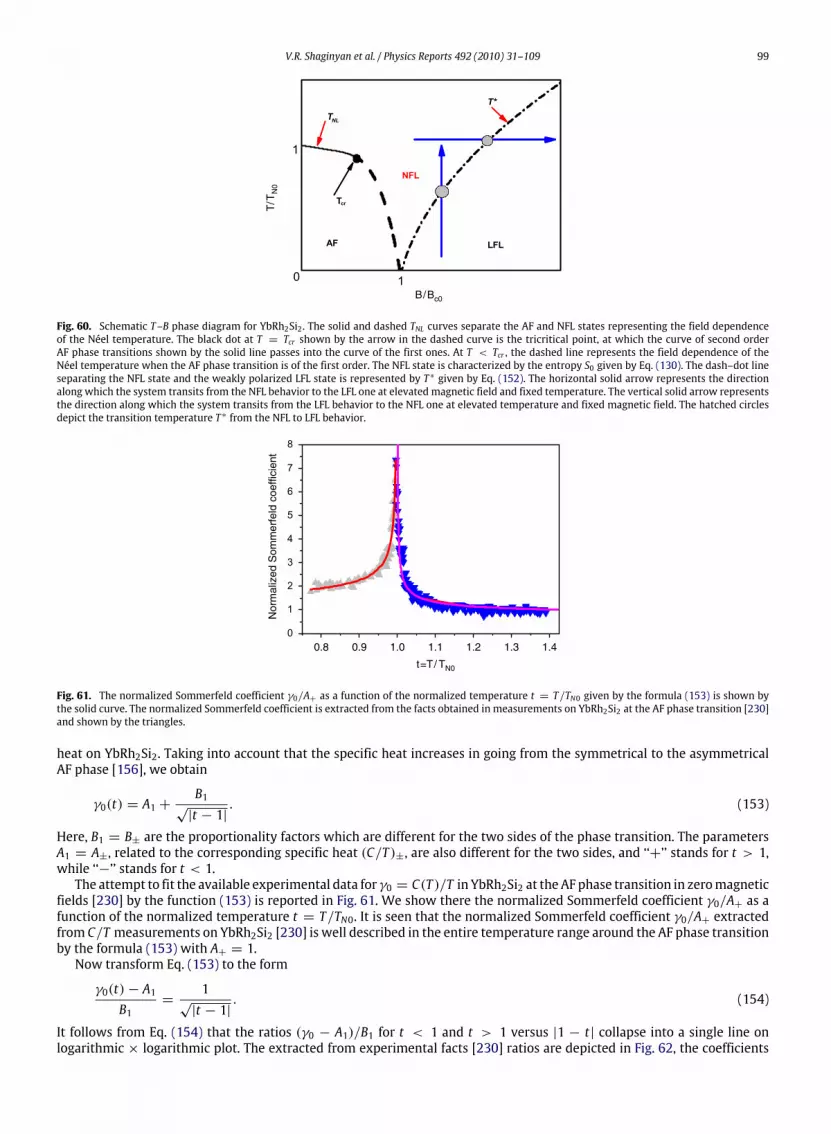
14.1. T–B phase diagram for YbRh2Si2 versus one for CeCoIn5 ........................................................................................................ 9814.2. The tricritical point in the B–T phase diagram of YbRh2Si2 ..................................................................................................... 9814.3. Entropy in YbRh2Si2 at low temperatures ................................................................................................................................ 100
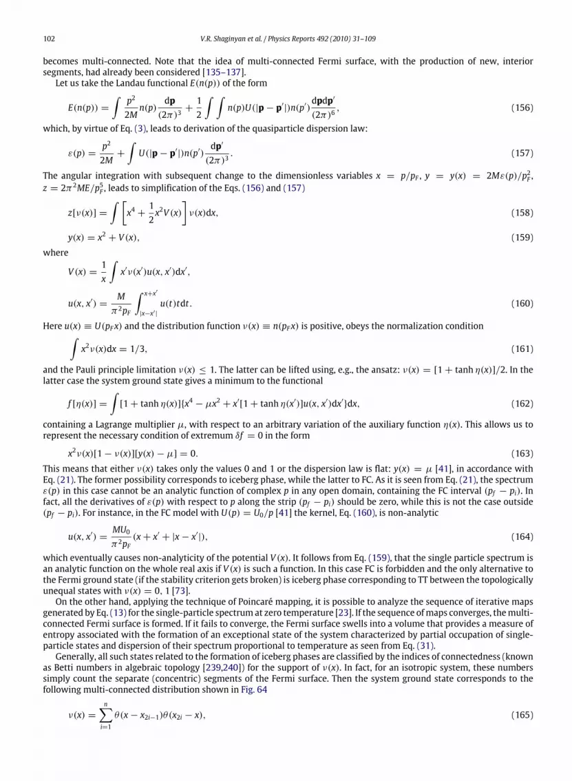
15. Topological phase transitions related to FCQPT.................................................................................................................................... 10116. Conclusions.............................................................................................................................................................................................. 105
Strongly correlated Fermi systems, such as heavy fermion (HF) metals, high-Tc superconductors, and two-dimensional(2D) Fermi liquids, are among themost intriguing andbest experimentally studied fundamental systems in physics. Howeveruntil very recently lacked theoretical explanations. The properties of these materials differ dramatically from those ofordinary Fermi systems [1–12]. For instance, in the case of metals with heavy fermions, the strong correlation of electronsleads to a renormalization of the effective mass of quasiparticles, which may exceed the ordinary, ‘‘bare’’, mass by severalorders of magnitude or even become infinitely large. The effective mass strongly depends on the temperature, pressure,or applied magnetic field. Such metals exhibit NFL behavior and unusual power laws of the temperature dependence ofthe thermodynamic properties at low temperatures. Ideas based on quantum and thermal fluctuations taking place at aquantum critical point (QCP) have been put forward and the fascinating behavior of these systems known as the non-Fermi
liquid (NFL) behavior was attributed to the fluctuations [1,3,13–17]. Suggested to describe one property, the ideas failed todo the same with the others and there was a real crisis and a new quantum phase transition responsible for the observedbehavior was required [7–11,13,18].The Landau theory of the Fermi liquid has a long history and remarkable results in describing a multitude of properties
of the electron liquid in ordinary metals and Fermi liquids of the 3He type [19–21]. The theory is based on the assumptionthat elementary excitations determine the physics at low temperatures. These excitations behave as quasiparticles, have acertain effective mass, and, judging by their basic properties, belong to the class of quasiparticles of a weakly interactingFermi gas. Hence, the effective mass M∗ is independent of the temperature, pressure, and magnetic field strength and is aparameter of the theory.The Landau Fermi liquid (LFL) theory fails to explain the results of experimental observations related to the dependence
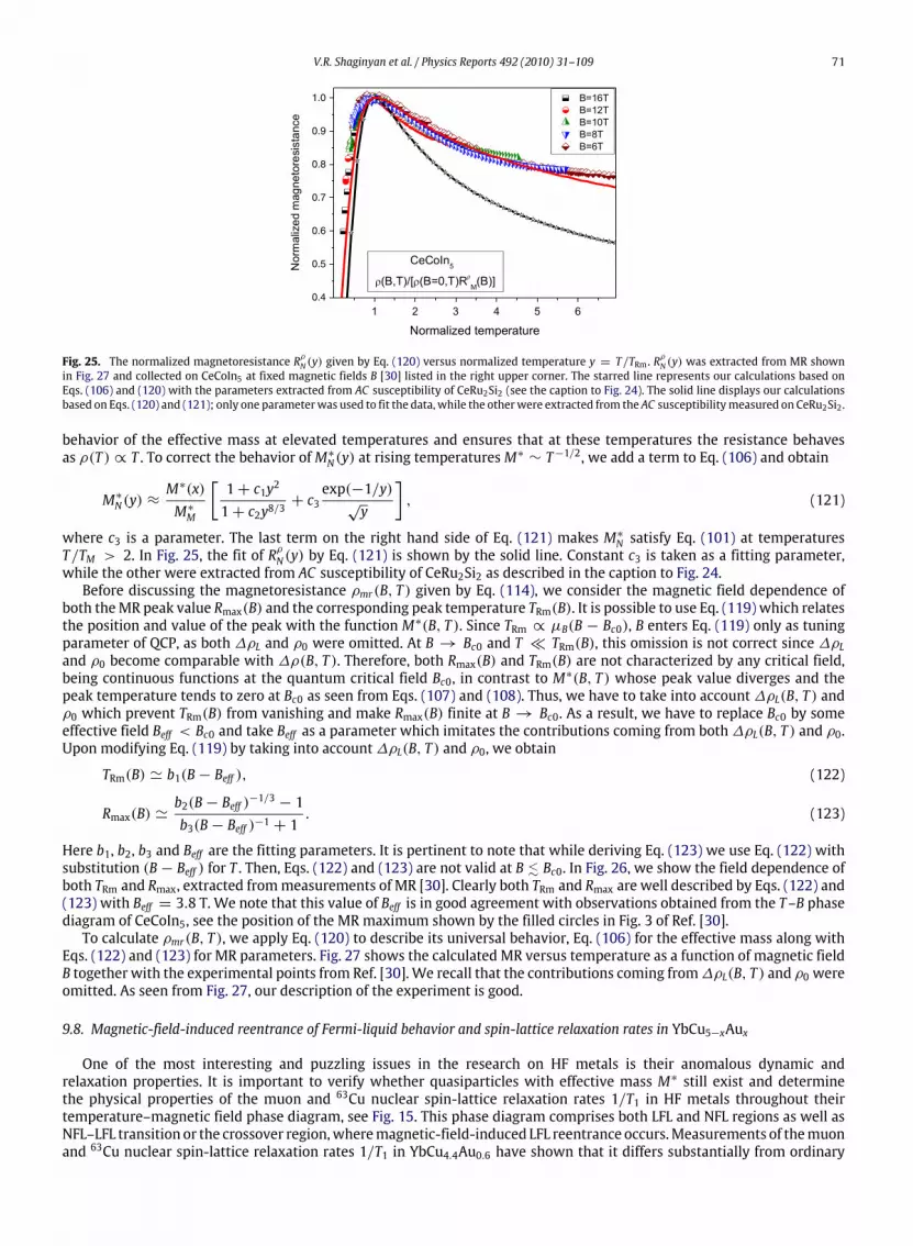
ofM∗ on the temperature T , magnetic field B, pressure, etc.; this has led to the conclusion that quasiparticles do not survivein strongly correlated Fermi systems and that the heavy electron does not retain its identity as a quasiparticle excitation[7–13,18].
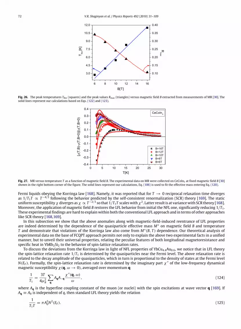
1.1. Quantum phase transitions and the non-Fermi liquid behavior of correlated Fermi systems
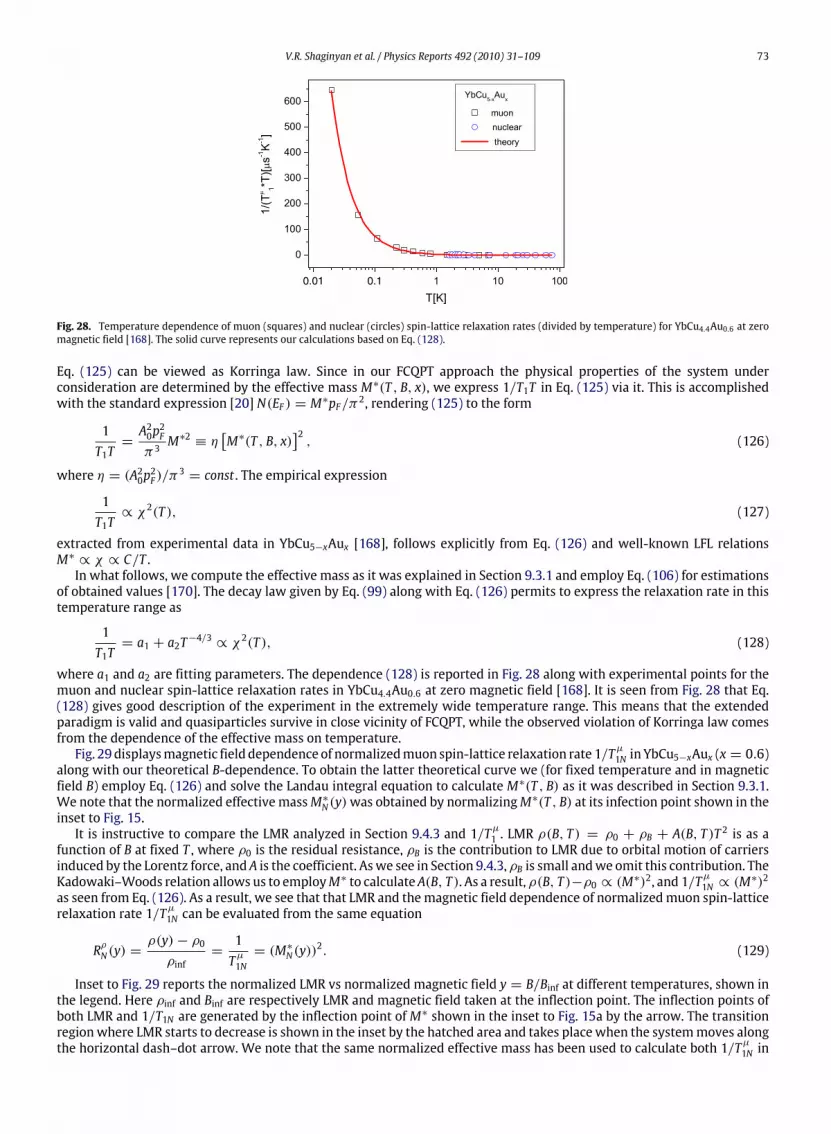
The unusual properties and NFL behavior observed in high-Tc superconductors, HF metals and 2D Fermi systems areassumed to be determined by various magnetic quantum phase transitions [1–9,11–14]. Since a quantum phase transitionoccurs at the temperature T = 0, the control parameters are the composition, electron (hole) number density x, pressure,magnetic field strength B, etc. A quantum phase transition occurs at a quantum critical point, which separates the orderedphase that emerges as a result of quantum phase transition from the disordered phase. It is usually assumed that magnetic(e.g., ferromagnetic and antiferromagnetic) quantum phase transitions are responsible for the NFL behavior. The criticalpoint of such a phase transition can be shifted to absolute zero by varying the above parameters.Universal behavior can be expected only if the system under consideration is very close to a quantum critical
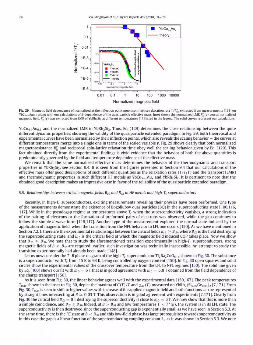
point, e.g., when the correlation length is much longer than the microscopic length scale, and critical quantum andthermal fluctuations determine the anomalous contribution to the thermodynamic functions of the metal. Quantum phasetransitions of this type are sowidespread [2–4,9–13] that we call them ordinary quantumphase transitions [22]. In this case,the physics of the phenomenon is determined by thermal and quantum fluctuations of the critical state, while quasiparticleexcitations are destroyed by these fluctuations. Conventional arguments that quasiparticles in strongly correlated Fermiliquids ‘‘get heavy and die’’ at a quantum critical point commonly employ thewell-known formula based on the assumptionsthat the z-factor (the quasiparticle weight in the single-particle state) vanishes at the points of second-order phasetransitions [18]. However, it has been shown that this scenario is problematic [23,24].The fluctuations in the order parameter developing an infinite correlation and the absence of quasiparticle excitations is
considered themain reason for the NFL behavior of heavy-fermionmetals, 2D fermion systems and high-Tc superconductors[3,4,9,12,13,25]. This approach faces certain difficulties, however. Critical behavior in experiments with metals containingheavy fermions is observed at high temperatures comparable to the effective Fermi temperature Tk. For instance, the thermalexpansion coefficient α(T ), which is a linear function of temperature for normal LFL, α(T ) ∝ T , demonstrates the
√T
temperature dependence in measurements involving CeNi2Ge2 as the temperature varies by two orders of magnitude (as itdecreases from 6 K to at least 50 mK) [14]. Such behavior can hardly be explained within the framework of the critical pointfluctuation theory. Obviously, such a situation is possible only as T → 0, when the critical fluctuations make the leadingcontribution to the entropy and when the correlation length is much longer than the microscopic length scale. At a certaintemperature Tk, this macroscopically large correlation length must be destroyed by ordinary thermal fluctuations and thecorresponding universal behavior must disappear.Another difficulty is in explaining the restoration of the LFL behavior under the application ofmagnetic fieldB, as observed
in HF metals and in high-Tc superconductors [1,15,26]. For the LFL state as T → 0, the electric resistivity ρ(T ) = ρ0 + AT 2,the heat capacity C(T ) = γ0T , and the magnetic susceptibility χ = const . It turns out that the coefficient A(B), theSommerfeld coefficient γ0(B) ∝ M∗, and themagnetic susceptibility χ(B) depend on themagnetic field strength B such thatA(B) ∝ γ 20 (B) and A(B) ∝ χ
2(B), which implies that the Kadowaki–Woods relation K = A(B)/γ 20 (B) [27] is B-independentand is preserved [15]. Such universal behavior, quite natural when quasiparticles with the effective mass M∗ playing themain role, can hardly be explained within the framework of the approach that presupposes the absence of quasiparticles,which is characteristic of ordinary quantum phase transitions in the vicinity of QCP. Indeed, there is no reason to expect thatγ0, χ and A are affected by the fluctuations in a correlated fashion.For instance, the Kadowaki–Woods relation does not agree with the spin density wave scenario [15] and with the results
of research in quantum criticality based on the renormalization-group approach [28]. Moreover, measurements of chargeand heat transfer have shown that the Wiedemann–Franz law holds in some high-Tc superconductors [26,29] and HFmetals [30–33]. All this suggests that quasiparticles do exist in such metals, and this conclusion is also corroborated byphotoemission spectroscopy results [34,35].The inability to explain the behavior of heavy-fermion metals while staying within the framework of theories based on
ordinary quantum phase transitions implies that another important concept introduced by Landau, the order parameter,also ceases to operate (e.g., see Refs. [9,11,18,13]). Thus, we are left without the most fundamental principles of many-body
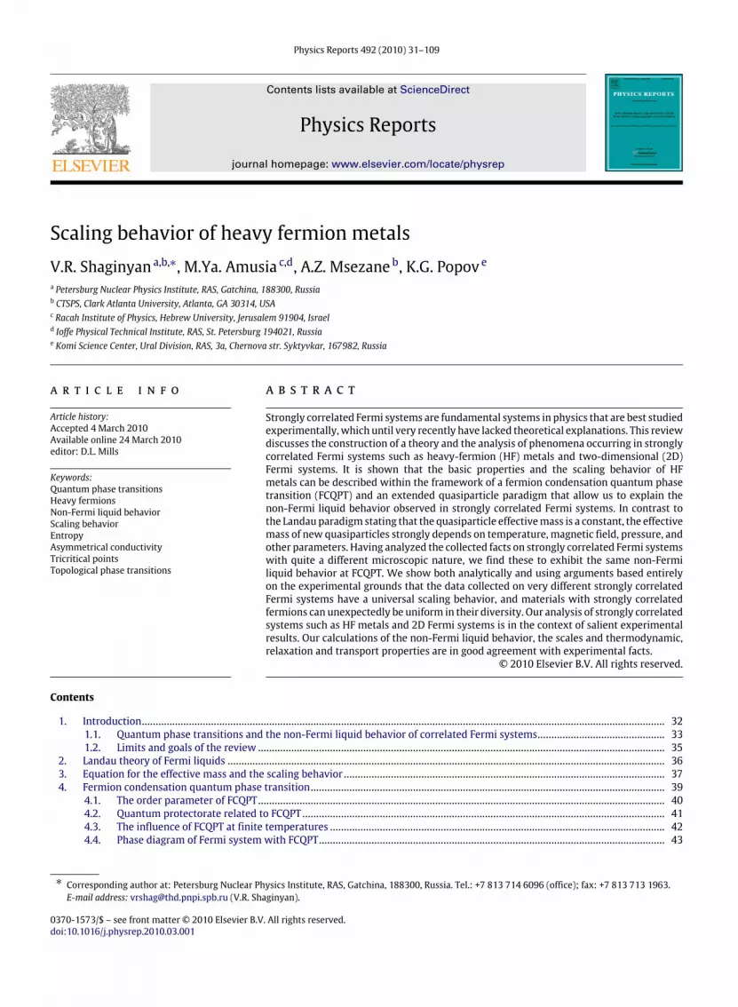
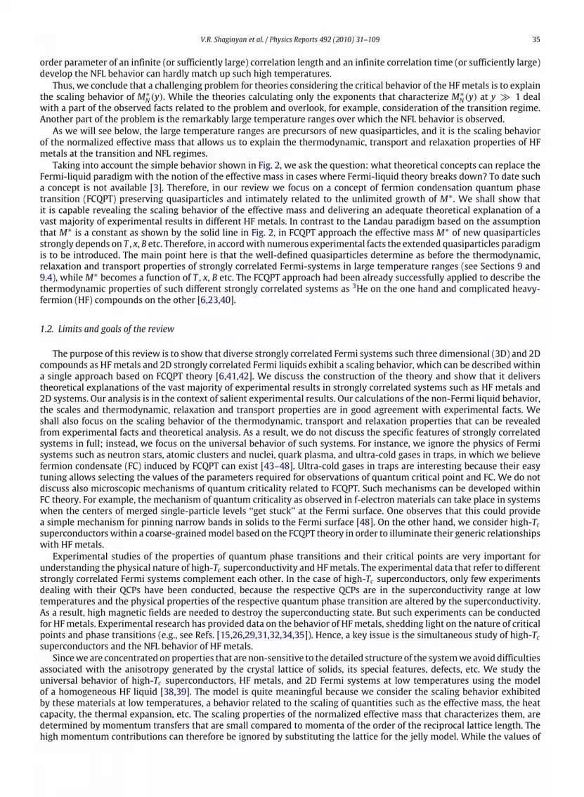
Fig. 1. Electronic specific heat of YbRh2Si2 , C/T , versus temperature T as a function of magnetic field B [36] shown in the legend.
.
.
.
..
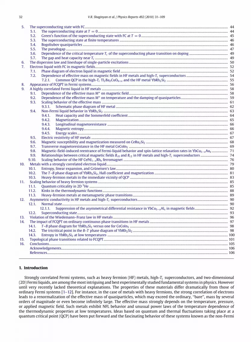
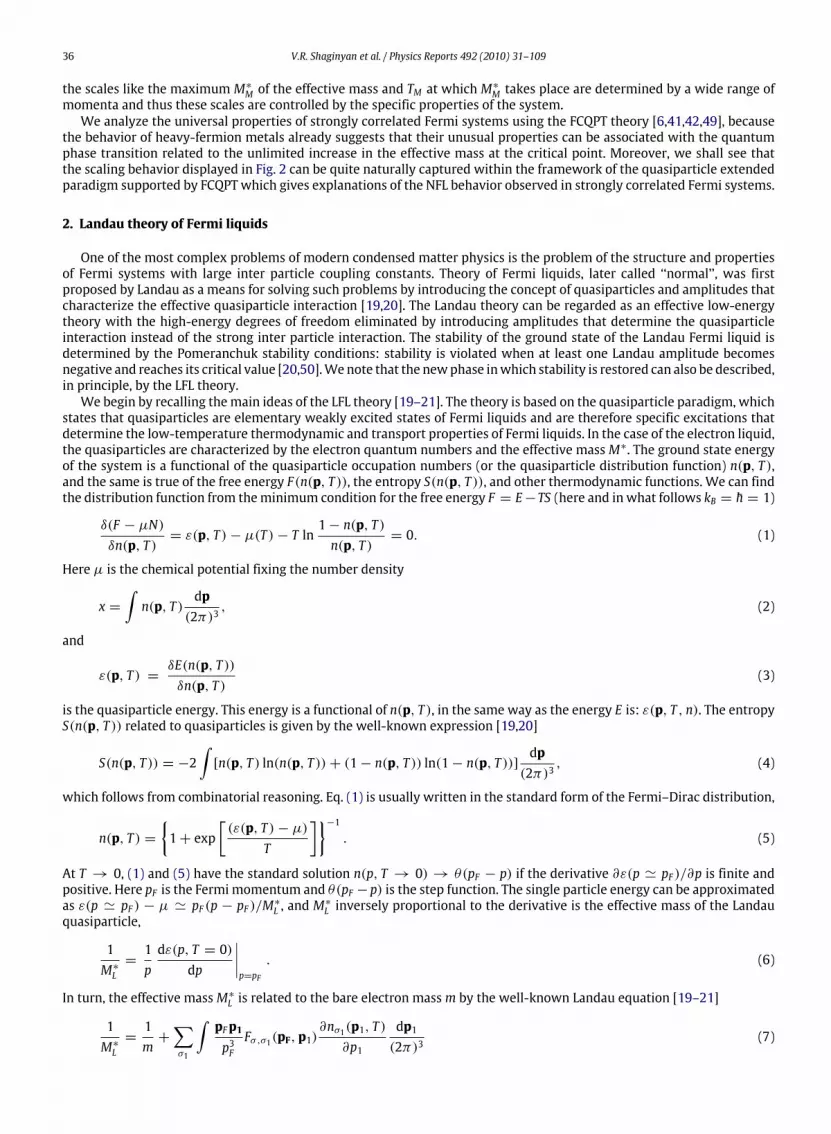
Fig. 2. The normalized effectivemassM∗N versus normalized temperature TN .M∗
N is extracted from themeasurements of the specific heat C/T on YbRh2Si2in magnetic fields B [36] listed in the legend. Constant effective massM∗L inherent in normal Landau Fermi liquids is depicted by the solid line.
quantum physics [19–21], and many interesting phenomena associated with the NFL behavior of strongly correlated Fermisystems remain unexplained.NFL behavior manifests itself in the power-law behavior of the physical quantities of strongly correlated Fermi systems
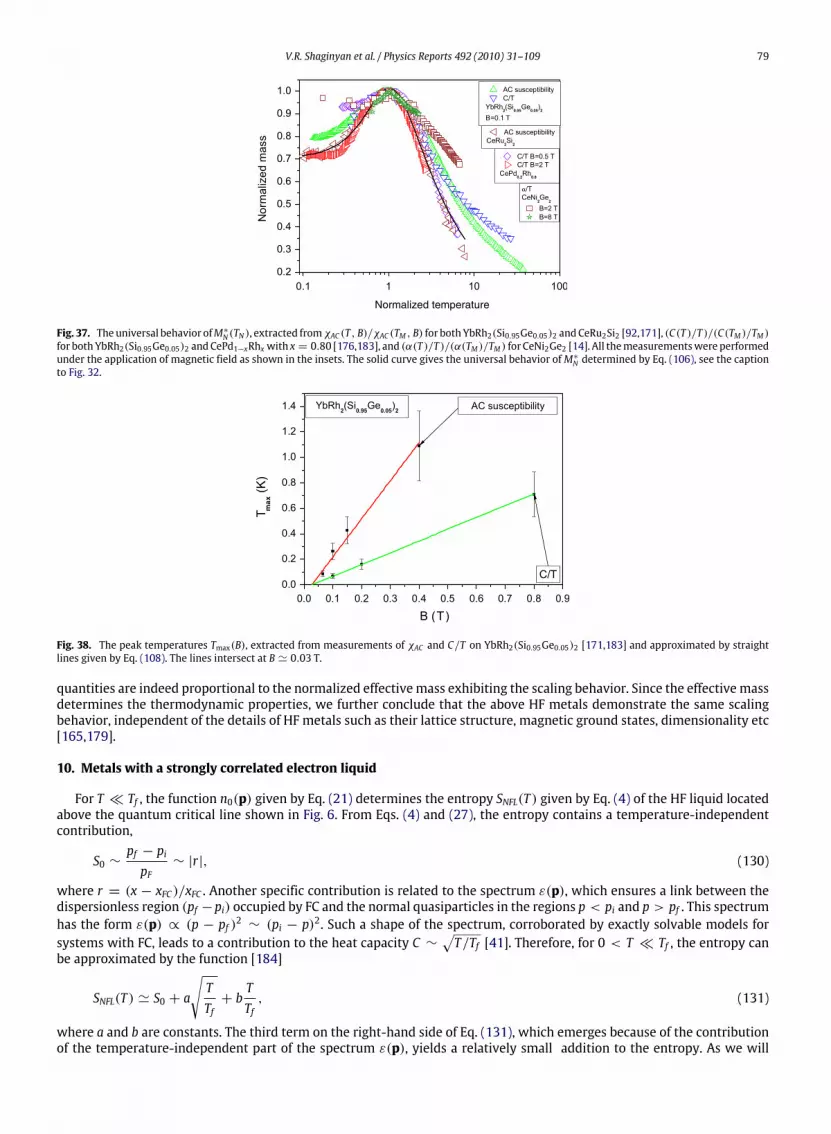
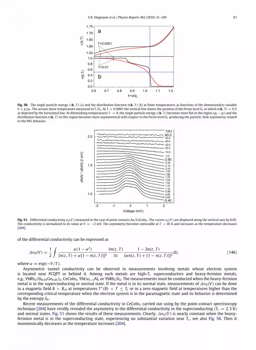
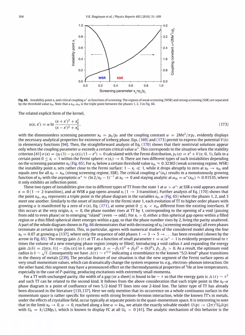
located close to their QCPs, with exponents different from those of a Fermi liquid [36,37]. It is common belief that the mainoutput of theory is the explanation of these exponents which are at least depended on the magnetic character of QCP anddimensionality of the system. On the other hand, the NFL behavior cannot be captured by these exponents as seen fromFig. 1. Indeed, the specific heat C/T exhibits a behavior that is to be described as a function of both temperature T andmagnetic B field rather than by a single exponent. One can see that at low temperatures C/T demonstrates the LFL behaviorwhich is changed by the transition regime at which C/T reaches its maximum and finally C/T decays into NFL behavior as afunction of T at fixed B. It is clearly seen from Fig. 1 that, in particularly in the transition regime, these exponents may havelittle physical significance.In order to show that the behavior of C/T displayed in Fig. 1 is of generic character, we remember that in the vicinity of
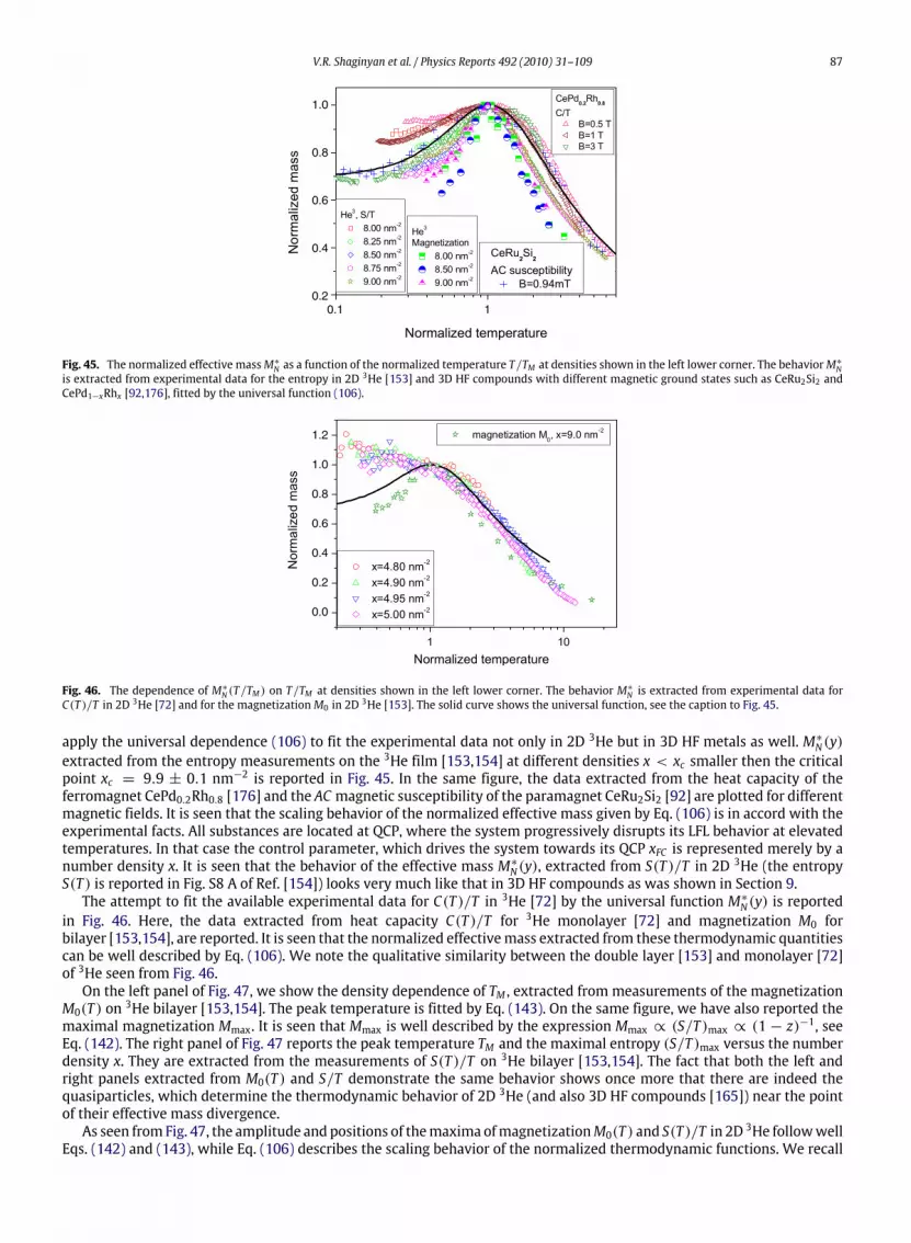
QCP it is helpful to use ‘‘internal’’ scales to measure the effective massM∗ ∝ C/T and temperature T [38,39]. As seen fromFig. 1, a maximum structure in C/T ∝ M∗M at temperature TM appears under the application of magnetic field B and TM shiftsto higher T as B is increased. The value of the Sommerfeld coefficient C/T = γ0 is saturated towards lower temperaturesdecreasing at elevated magnetic field. To obtain the normalized effective massM∗N , we useM
∗
M and TM as ‘‘internal’’ scales:Themaximumstructure in C/T was used to normalize C/T , and T was normalized by TM . In Fig. 2 the obtainedM∗N = M
∗/M∗Mas a function of normalized temperature TN = T/TM is shown by geometrical figures. Note that we have excluded theexperimental data taken in magnetic field B = 0.06 T. In that case, as will be shown in Sections 9.3 and 9.4.5, TM → 0and the corresponding TM andM∗M are unavailable. It is seen that the LFL state and NFL one are separated by the transitionregime at whichM∗N reaches its maximum value. Fig. 2 reveals the scaling behavior of the normalized experimental curves— the curves at different magnetic fields B merge into a single one in terms of the normalized variable y = T/TM . As seenfrom Fig. 2, the normalized effective massM∗N(y) extracted from the measurements is not a constant, as would be for a LFL,and shows the scaling behavior over three decades in normalized temperature y. It is seen from Figs. 1 and 2 that the NFLbehavior and the associated scaling extend at least to temperatures up to few Kelvins. Scenario where fluctuations in the
order parameter of an infinite (or sufficiently large) correlation length and an infinite correlation time (or sufficiently large)develop the NFL behavior can hardly match up such high temperatures.Thus, we conclude that a challenging problem for theories considering the critical behavior of the HFmetals is to explain
the scaling behavior of M∗N(y). While the theories calculating only the exponents that characterize M∗
N(y) at y 1 dealwith a part of the observed facts related to the problem and overlook, for example, consideration of the transition regime.Another part of the problem is the remarkably large temperature ranges over which the NFL behavior is observed.As we will see below, the large temperature ranges are precursors of new quasiparticles, and it is the scaling behavior
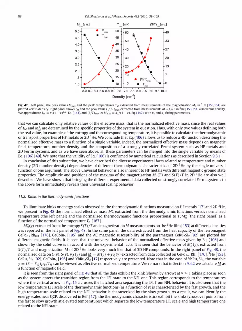
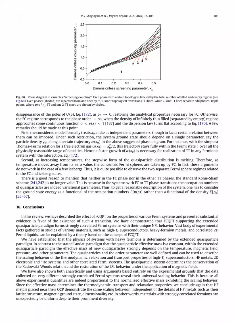
of the normalized effective mass that allows us to explain the thermodynamic, transport and relaxation properties of HFmetals at the transition and NFL regimes.Taking into account the simple behavior shown in Fig. 2, we ask the question: what theoretical concepts can replace the
Fermi-liquid paradigmwith the notion of the effective mass in cases where Fermi-liquid theory breaks down? To date sucha concept is not available [3]. Therefore, in our review we focus on a concept of fermion condensation quantum phasetransition (FCQPT) preserving quasiparticles and intimately related to the unlimited growth of M∗. We shall show thatit is capable revealing the scaling behavior of the effective mass and delivering an adequate theoretical explanation of avast majority of experimental results in different HF metals. In contrast to the Landau paradigm based on the assumptionthat M∗ is a constant as shown by the solid line in Fig. 2, in FCQPT approach the effective mass M∗ of new quasiparticlesstrongly depends on T , x, B etc. Therefore, in accordwith numerous experimental facts the extended quasiparticles paradigmis to be introduced. The main point here is that the well-defined quasiparticles determine as before the thermodynamic,relaxation and transport properties of strongly correlated Fermi-systems in large temperature ranges (see Sections 9 and9.4), whileM∗ becomes a function of T , x, B etc. The FCQPT approach had been already successfully applied to describe thethermodynamic properties of such different strongly correlated systems as 3He on the one hand and complicated heavy-fermion (HF) compounds on the other [6,23,40].
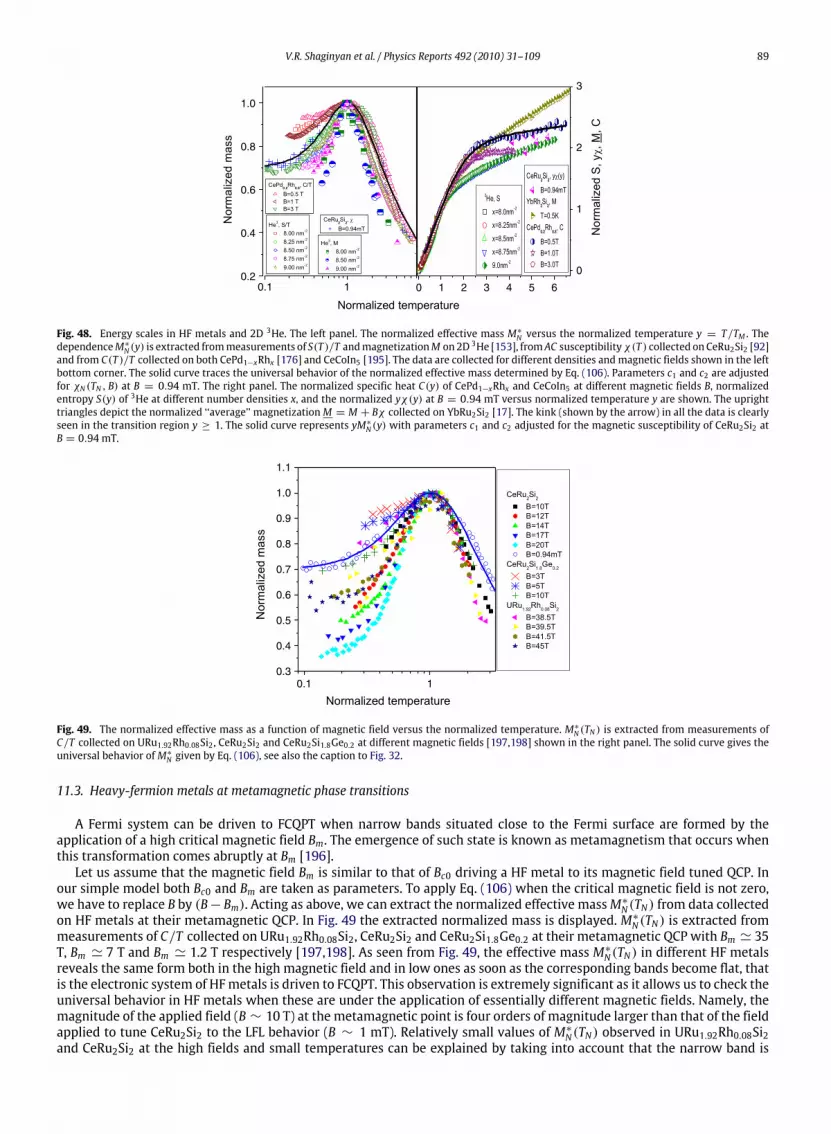
1.2. Limits and goals of the review
The purpose of this review is to show that diverse strongly correlated Fermi systems such three dimensional (3D) and 2Dcompounds as HFmetals and 2D strongly correlated Fermi liquids exhibit a scaling behavior, which can be described withina single approach based on FCQPT theory [6,41,42]. We discuss the construction of the theory and show that it deliverstheoretical explanations of the vast majority of experimental results in strongly correlated systems such as HF metals and2D systems. Our analysis is in the context of salient experimental results. Our calculations of the non-Fermi liquid behavior,the scales and thermodynamic, relaxation and transport properties are in good agreement with experimental facts. Weshall also focus on the scaling behavior of the thermodynamic, transport and relaxation properties that can be revealedfrom experimental facts and theoretical analysis. As a result, we do not discuss the specific features of strongly correlatedsystems in full; instead, we focus on the universal behavior of such systems. For instance, we ignore the physics of Fermisystems such as neutron stars, atomic clusters and nuclei, quark plasma, and ultra-cold gases in traps, in which we believefermion condensate (FC) induced by FCQPT can exist [43–48]. Ultra-cold gases in traps are interesting because their easytuning allows selecting the values of the parameters required for observations of quantum critical point and FC. We do notdiscuss also microscopic mechanisms of quantum criticality related to FCQPT. Such mechanisms can be developed withinFC theory. For example, the mechanism of quantum criticality as observed in f-electron materials can take place in systemswhen the centers of merged single-particle levels ‘‘get stuck’’ at the Fermi surface. One observes that this could providea simple mechanism for pinning narrow bands in solids to the Fermi surface [48]. On the other hand, we consider high-Tcsuperconductors within a coarse-grainedmodel based on the FCQPT theory in order to illuminate their generic relationshipswith HF metals.Experimental studies of the properties of quantum phase transitions and their critical points are very important for
understanding the physical nature of high-Tc superconductivity and HFmetals. The experimental data that refer to differentstrongly correlated Fermi systems complement each other. In the case of high-Tc superconductors, only few experimentsdealing with their QCPs have been conducted, because the respective QCPs are in the superconductivity range at lowtemperatures and the physical properties of the respective quantum phase transition are altered by the superconductivity.As a result, high magnetic fields are needed to destroy the superconducting state. But such experiments can be conductedfor HFmetals. Experimental research has provided data on the behavior of HFmetals, shedding light on the nature of criticalpoints and phase transitions (e.g., see Refs. [15,26,29,31,32,34,35]). Hence, a key issue is the simultaneous study of high-Tcsuperconductors and the NFL behavior of HF metals.Sincewe are concentrated onproperties that are non-sensitive to the detailed structure of the systemweavoid difficulties
associated with the anisotropy generated by the crystal lattice of solids, its special features, defects, etc. We study theuniversal behavior of high-Tc superconductors, HF metals, and 2D Fermi systems at low temperatures using the modelof a homogeneous HF liquid [38,39]. The model is quite meaningful because we consider the scaling behavior exhibitedby these materials at low temperatures, a behavior related to the scaling of quantities such as the effective mass, the heatcapacity, the thermal expansion, etc. The scaling properties of the normalized effective mass that characterizes them, aredetermined by momentum transfers that are small compared to momenta of the order of the reciprocal lattice length. Thehigh momentum contributions can therefore be ignored by substituting the lattice for the jelly model. While the values of
the scales like the maximum M∗M of the effective mass and TM at which M∗
M takes place are determined by a wide range ofmomenta and thus these scales are controlled by the specific properties of the system.We analyze the universal properties of strongly correlated Fermi systems using the FCQPT theory [6,41,42,49], because
the behavior of heavy-fermion metals already suggests that their unusual properties can be associated with the quantumphase transition related to the unlimited increase in the effective mass at the critical point. Moreover, we shall see thatthe scaling behavior displayed in Fig. 2 can be quite naturally captured within the framework of the quasiparticle extendedparadigm supported by FCQPT which gives explanations of the NFL behavior observed in strongly correlated Fermi systems.
2. Landau theory of Fermi liquids
One of the most complex problems of modern condensed matter physics is the problem of the structure and propertiesof Fermi systems with large inter particle coupling constants. Theory of Fermi liquids, later called ‘‘normal’’, was firstproposed by Landau as a means for solving such problems by introducing the concept of quasiparticles and amplitudes thatcharacterize the effective quasiparticle interaction [19,20]. The Landau theory can be regarded as an effective low-energytheory with the high-energy degrees of freedom eliminated by introducing amplitudes that determine the quasiparticleinteraction instead of the strong inter particle interaction. The stability of the ground state of the Landau Fermi liquid isdetermined by the Pomeranchuk stability conditions: stability is violated when at least one Landau amplitude becomesnegative and reaches its critical value [20,50].Wenote that the newphase inwhich stability is restored can also be described,in principle, by the LFL theory.We begin by recalling themain ideas of the LFL theory [19–21]. The theory is based on the quasiparticle paradigm, which
states that quasiparticles are elementary weakly excited states of Fermi liquids and are therefore specific excitations thatdetermine the low-temperature thermodynamic and transport properties of Fermi liquids. In the case of the electron liquid,the quasiparticles are characterized by the electron quantum numbers and the effective massM∗. The ground state energyof the system is a functional of the quasiparticle occupation numbers (or the quasiparticle distribution function) n(p, T ),and the same is true of the free energy F(n(p, T )), the entropy S(n(p, T )), and other thermodynamic functions. We can findthe distribution function from theminimum condition for the free energy F = E−TS (here and in what follows kB = h = 1)
δ(F − µN)δn(p, T )
= ε(p, T )− µ(T )− T ln1− n(p, T )n(p, T )
= 0. (1)
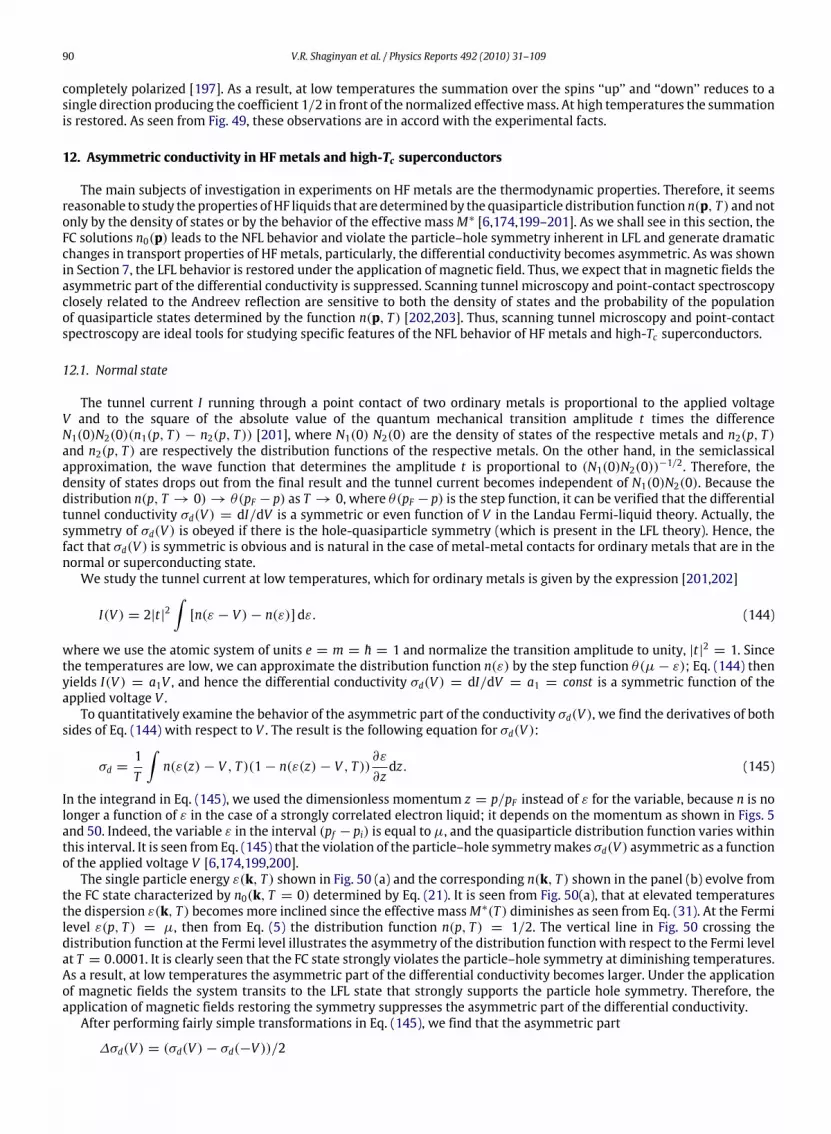
Here µ is the chemical potential fixing the number density
x =∫n(p, T )
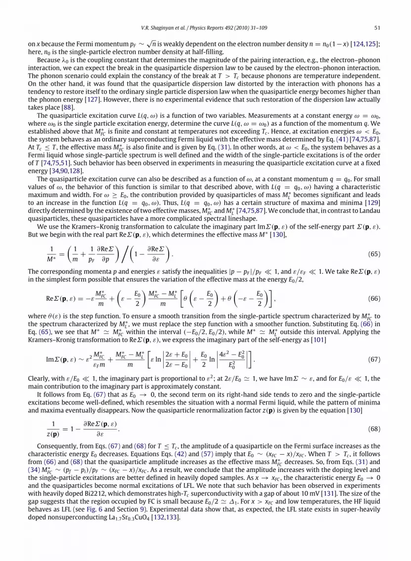
dp(2π)3
, (2)
and
ε(p, T ) =δE(n(p, T ))δn(p, T )
(3)
is the quasiparticle energy. This energy is a functional of n(p, T ), in the same way as the energy E is: ε(p, T , n). The entropyS(n(p, T )) related to quasiparticles is given by the well-known expression [19,20]
S(n(p, T )) = −2∫[n(p, T ) ln(n(p, T ))+ (1− n(p, T )) ln(1− n(p, T ))]
dp(2π)3
, (4)
which follows from combinatorial reasoning. Eq. (1) is usually written in the standard form of the Fermi–Dirac distribution,
n(p, T ) =1+ exp
[(ε(p, T )− µ)
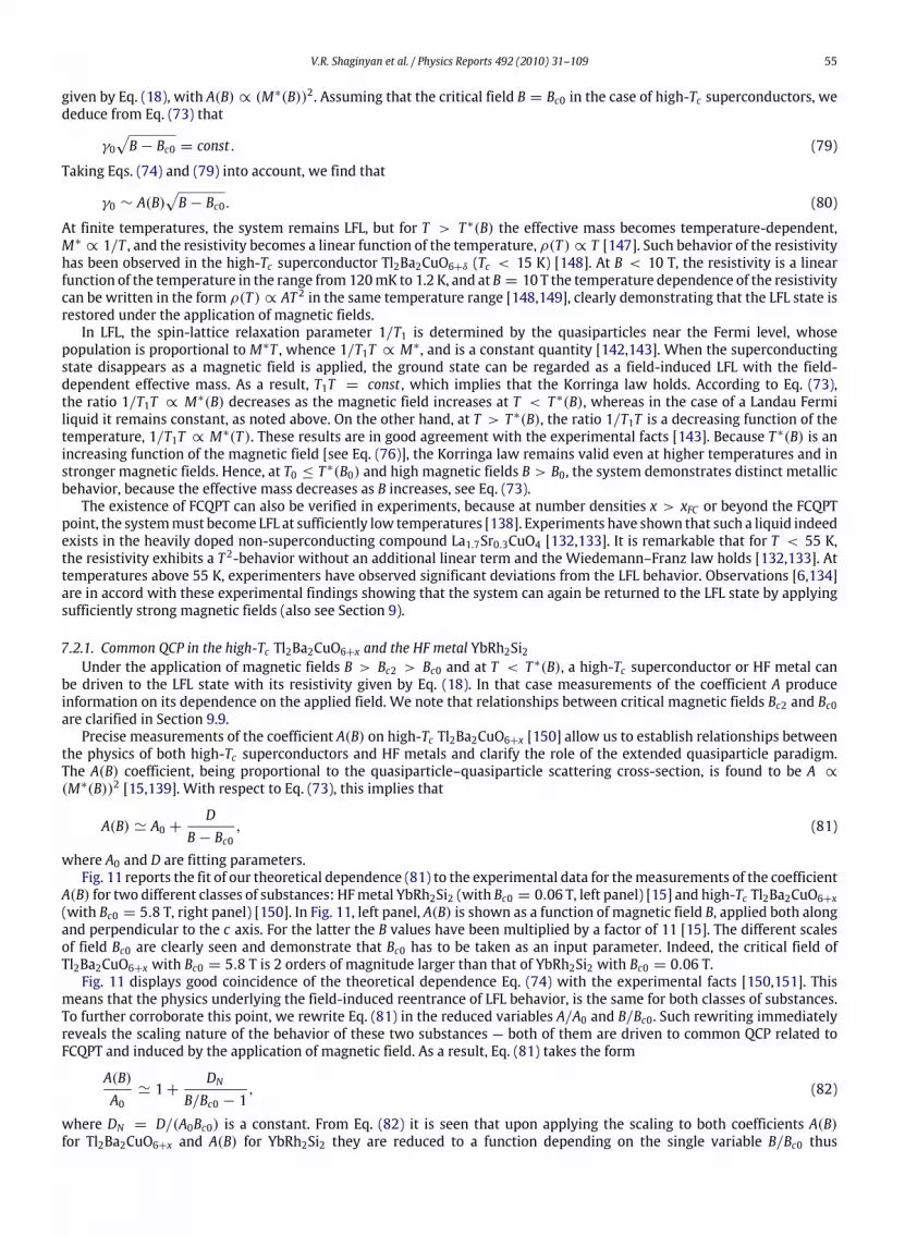
T
]−1. (5)
At T → 0, (1) and (5) have the standard solution n(p, T → 0) → θ(pF − p) if the derivative ∂ε(p ' pF )/∂p is finite andpositive. Here pF is the Fermi momentum and θ(pF −p) is the step function. The single particle energy can be approximatedas ε(p ' pF ) − µ ' pF (p − pF )/M∗L , and M
∗
L inversely proportional to the derivative is the effective mass of the Landauquasiparticle,
1M∗L=1pdε(p, T = 0)
dp
∣∣∣∣p=pF
. (6)
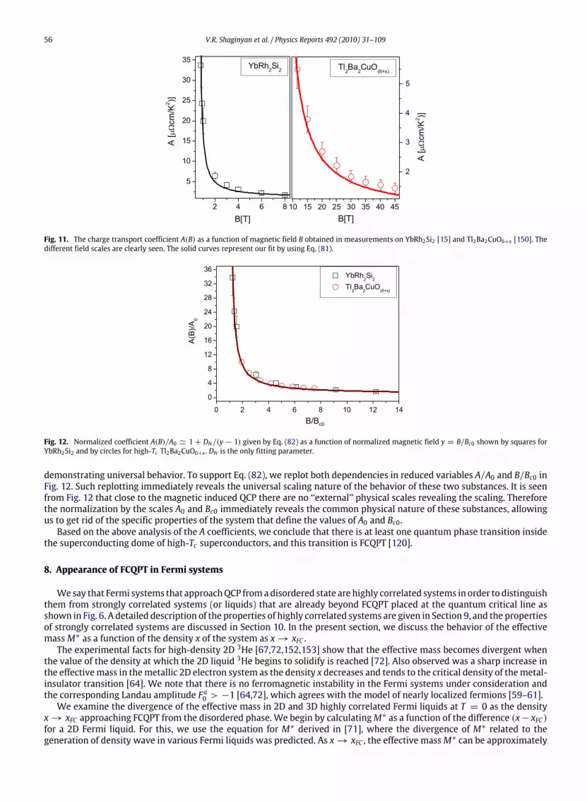
In turn, the effective massM∗L is related to the bare electron massm by the well-known Landau equation [19–21]
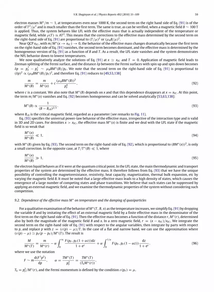
where Fσ ,σ1(pF, p1) is the Landau amplitude, which depends on the momenta pF and p and the spins σ . For simplicity,we ignore the spin dependence of the effective mass, because M∗L is almost completely spin-independent in the case of ahomogeneous liquid and weak magnetic fields. The Landau amplitude F is given by
Fσ ,σ1(p, p1, n) =δ2E(n)
δnσ (p)δnσ1(p1). (8)
The stability of the ground state of LFL is determined by the Pomeranchuk stability conditions: stability is violated when atleast one Landau amplitude becomes negative and reaches its critical value [20,21,50]
F a,sL = −(2L+ 1). (9)
Here F aL and FsL are the dimensionless spin-symmetric and spin-antisymmetric Landau amplitudes, L is the angular
momentum related to the corresponding Legendre polynomials PL,
F(pσ , p1σ1) =1N
∞∑L=0
PL(Θ)[F aL σ , σ1 + F
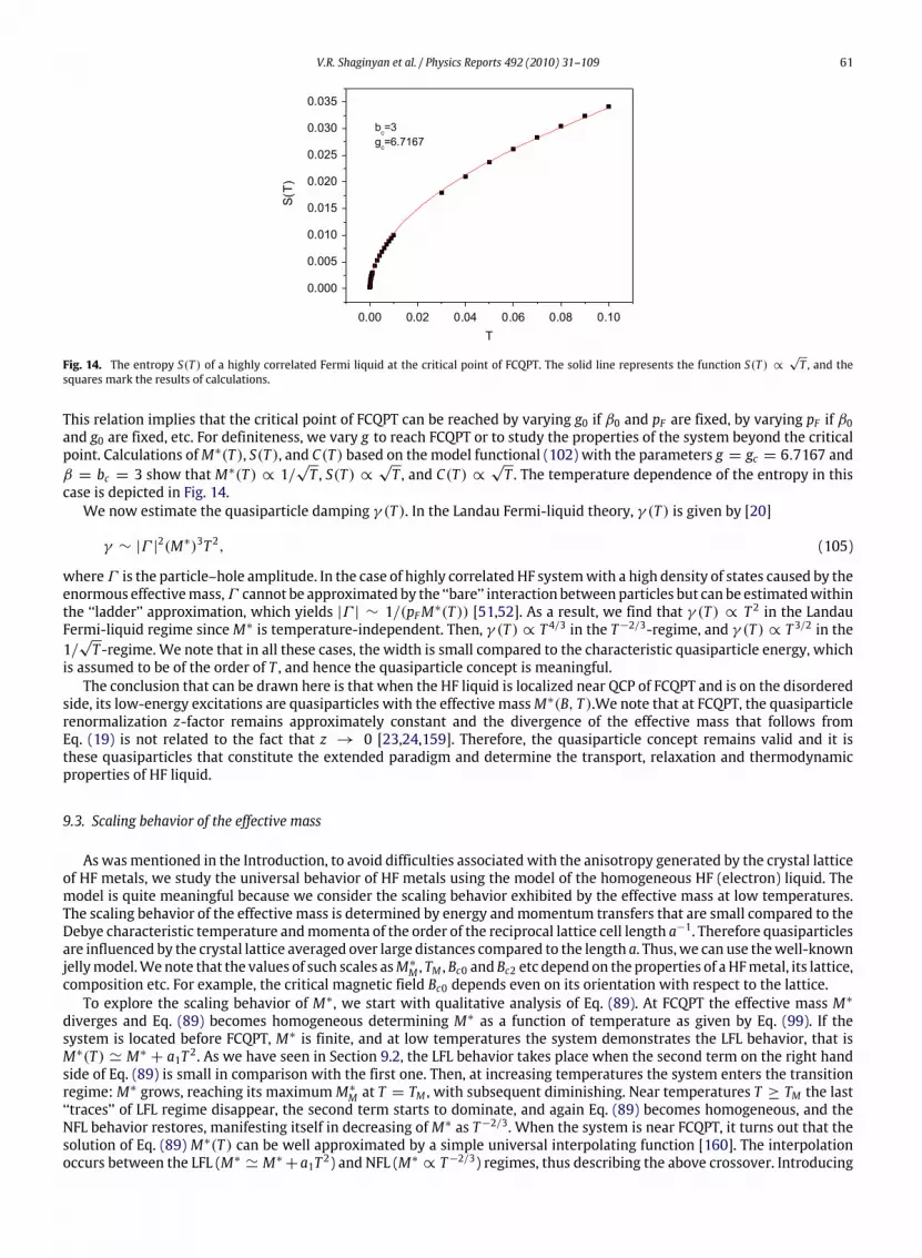
sL
]. (10)
HereΘ is the angle between momenta p and p1 and the density of states N = M∗L pF/(2π2). It follows from Eq. (7) that
M∗Lm= 1+
F s13. (11)
In accordance with the Pomeranchuk stability conditions it is seen from Eq. (11) that F s1 > −3, otherwise the effective massbecomes negative leading to unstable state when it is energetically favorable to excite quasiparticles near the Fermi surface.In what follows, we shall omit the spin indices σ for simplicity.To deal with the transport properties of Fermi systems, one needs a transport equation describing slowly varying
disturbances of the quasiparticle distribution function np(r, t) which depends on position r and time t . As long as thetransferred energy ω and momentum q of the quanta of external field are much smaller than the energy and momentumof the quasiparticles, qpF/(TM∗L ) 1 and ω/T 1, the quasiparticle distribution function n(q, ω) satisfies the transportequation [19–21]
∂np∂t+∇pεp∇rnp −∇rεp∇pnp = I[np]. (12)
The left-hand side of Eq. (12) describes the dissipationless dynamic of quasiparticles in phase space. The quasiparticleenergy εp(r, t) now depends on its position and time, and the collision integral I[np] measures the rate of change of thedistribution function due to collisions. The transport equation (12) allows one to derive all the transport properties andcollective excitations of a Fermi system.It is common belief that the equations of this subsection are phenomenological and inapplicable to describe Fermi
systems characterized by the effective mass M∗ strongly dependent on temperature, external magnetic fields B, pressureP etc. On the other hand, facts collected on HF metals demonstrate the specific behavior when the effective mass stronglydepends on temperature T , doping (or the number density) x and applied magnetic fields B, while the effective mass M∗itself can reach very high values or even diverge, see e.g. [3,4]. As we have seen in Section 1 such a behavior is so unusualthat the traditional Landau quasiparticles paradigm fails to describe it. Therefore, in accord with numerous experimentalfacts the extended quasiparticles paradigm is to be introduced with the well-defined quasiparticles determining as beforethe thermodynamic and transport properties of strongly correlated Fermi-systems,M∗ becomes a function of T , x, B, whilethe dependence of the effective mass on T , x, B gives rise to the NFL behavior [6,23,38,51–53].As we shall see in the following Section 3, Eq. (7) can be derived microscopically and it becomes compatible with the
extended paradigm.
3. Equation for the effective mass and the scaling behavior
Toderive the equationdetermining the effectivemass,we consider themodel of a homogeneousHF liquid and employ thedensity functional theory for superconductors (SCDFT) [54] which allows us to consider E as a functional of the occupationsnumbers n(p) [38,55–57]. As a result, the ground state energy of the normal state E becomes the functional of the occupationnumbers and the function of the number density x, E = E(n(p), x), while Eq. (3) gives the single-particle spectrum. Upondifferentiating both sides of Eq. (3)with respect to p and after some algebra and integration by parts, we obtain [23,38,55,56]
∂ε(p)∂p=pm+
∫F(p, p1, n)
∂n(p1)∂p1
dp1(2π)3
. (13)
To calculate the derivative ∂ε(p)/∂p, we employ the functional representation
It is seen directly from Eq. (13) that the effective mass is given by the well-known Landau equation
1M∗=1m+
∫pFp1p3FF(pF, p1, n)
∂n(p1)∂p1
dp1(2π)3
. (15)
For simplicity, we ignore the spin dependencies. To calculateM∗ as a function of T , we construct the free energy F = E− TS,where the entropy S is given by Eq. (4). Minimizing F with respect to n(p), we arrive at the Fermi–Dirac distribution, Eq. (5).Due to the above derivation, we conclude that Eqs. (13) and (15) are exact ones and allow us to calculate the behavior ofboth ∂ε(p)/∂p andM∗ which now is a function of temperature T , external magnetic field B, number density x and pressureP rather than a constant. As we will see it is this feature ofM∗ that forms both the scaling and the NFL behavior observed inmeasurements on HF metals.In LFL theory it is assumed thatM∗L is positive, finite and constant. As a result, the temperature-dependent corrections to
M∗L , the quasiparticle energy ε(p) and other quantities begin with the term proportional to T2 in 3D systems and with the
term proportional to T in 2D one [58]. The effective mass is given by Eq. (7), and the specific heat C is [19]
C =2π2NT3= γ0T = T
∂S∂T, (16)
and the spin susceptibility
χ =3γ0µ2B
π2(1+ F a0 ), (17)
whereµB is the Bohr magneton and γ0 ∝ M∗L . In the case of LFL, upon using the transport Eq. (12) one finds for the electricalresistivity at low T [21]
ρ(T ) = ρ0 + ATαR , (18)
where ρ0 is the residual resistivity, the exponent αR = 2 and A is the coefficient determining the charge transport. Thecoefficient is proportional to the quasiparticle–quasiparticle scattering cross-section. Eq. (18) symbolizes and defines theLFL behavior observed in normal metals.Eq. (15) at T = 0, combined with the fact that n(p, T = 0) becomes θ(pF − p), yields the well-known result [59–61]M∗
m=
11− F 1/3
where F 1 = N0f 1, N0 = mpF/(2π2) is the density of states of a free Fermi gas and f 1(pF , pF ) is the p-wave component of theLandau interaction amplitude. Because x = p3F/3π
2 in the Landau Fermi-liquid theory, the Landau interaction amplitudecan be written as F 1(pF , pF ) = F 1(x). Provided that at a certain critical point xFC , the denominator (1 − F 1(x)/3) tends tozero, i.e., (1− F 1(x)/3) ∝ (x− xFC )+ a(x− xFC )2 + · · · → 0, we find that [62,63]
M∗(x)m' a1 +
a2x− xFC
∝1r
(19)
where a1 and a2 are constants and r = (x − xFC )/xFC is the ‘‘distance’’ from QCP xFC at which M∗(x → xFC ) → ∞. Wenote that the divergence of the effective mass given by Eq. (19) does preserve the Pomeranchuk stability conditions for F 1positive, see Eq. (9). Eqs. (11) and (19) seem to be different but it is not the case since F 1 ∝ m, while F s1 ∝ M
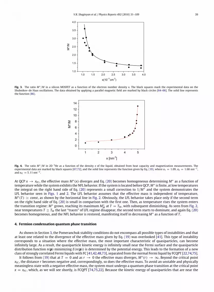
∗ and Eq. (11)represents an implicit formula for the effective mass.The behavior of M∗(x) described by formula (19) is in good agreement with the results of experiments [67,64,65] and
calculations [68–70]. In the case of electron systems, Eq. (19) holds for x > xFC , while for 2D 3He we have x < xFC so thatalways r > 0 [42,71] (see also Section 8). Such behavior of the effective mass is observed in HF metals, which have a fairlyflat and narrow conductivity band corresponding to a large effective mass, with a strong correlation and the effective Fermitemperature Tk ∼ p2F/M
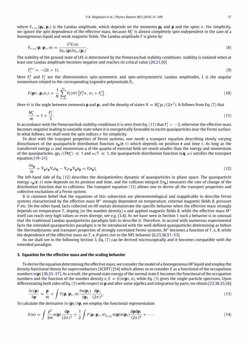
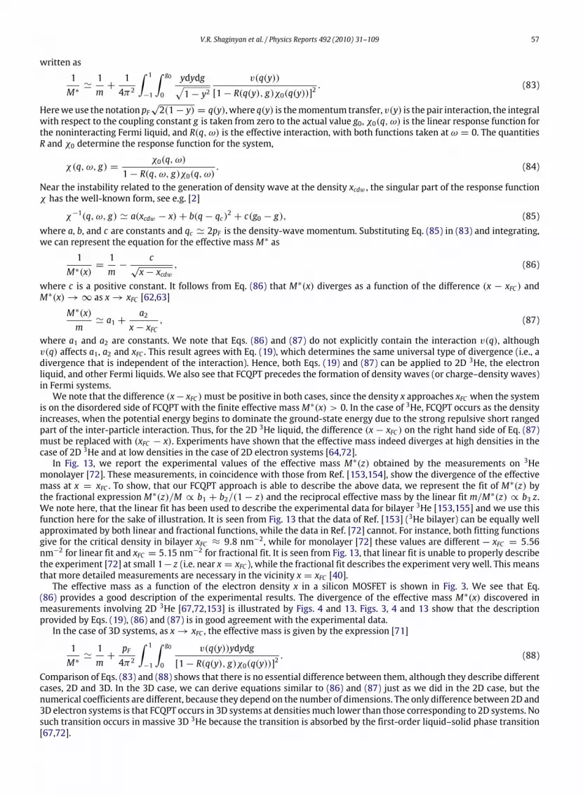
∗(x) of the order of several dozen degrees kelvin or even lower (e.g., see Ref. [1]).The effective mass as a function of the electron density x in a silicon MOSFET (Metal Oxide Semiconductor Field Effect
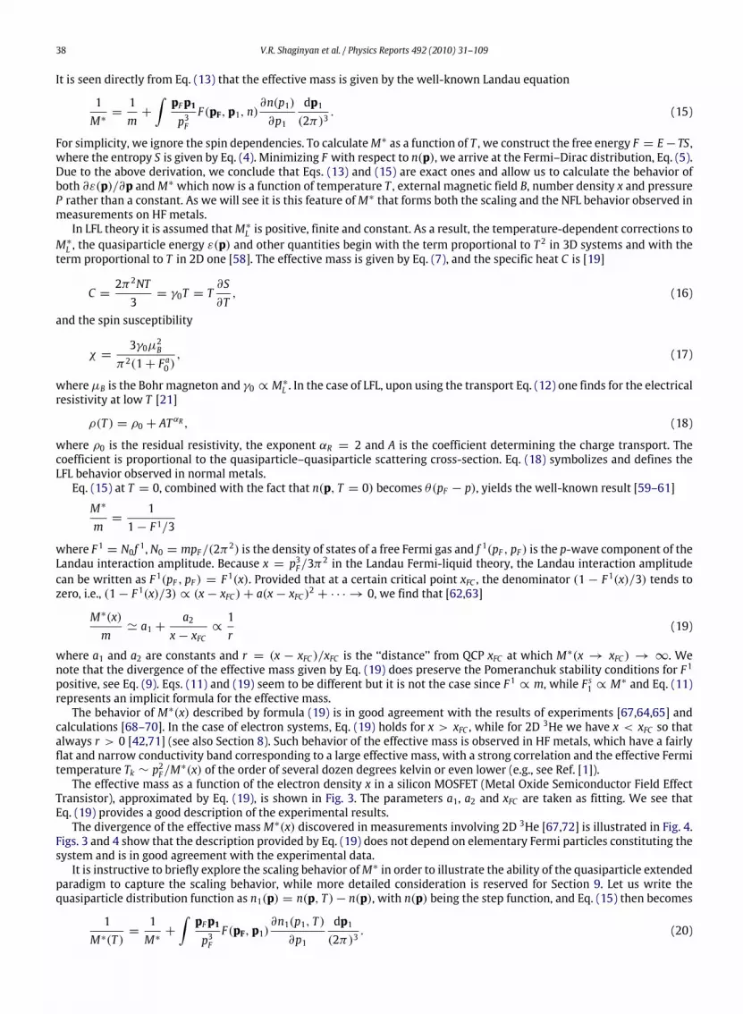
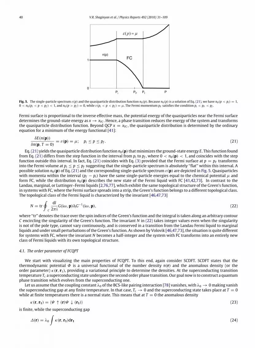
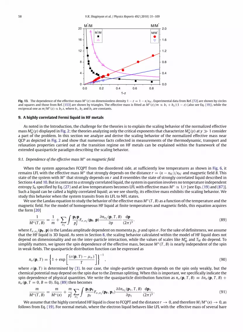
Transistor), approximated by Eq. (19), is shown in Fig. 3. The parameters a1, a2 and xFC are taken as fitting. We see thatEq. (19) provides a good description of the experimental results.The divergence of the effective massM∗(x) discovered in measurements involving 2D 3He [67,72] is illustrated in Fig. 4.
Figs. 3 and 4 show that the description provided by Eq. (19) does not depend on elementary Fermi particles constituting thesystem and is in good agreement with the experimental data.It is instructive to briefly explore the scaling behavior ofM∗ in order to illustrate the ability of the quasiparticle extended
paradigm to capture the scaling behavior, while more detailed consideration is reserved for Section 9. Let us write thequasiparticle distribution function as n1(p) = n(p, T )− n(p), with n(p) being the step function, and Eq. (15) then becomes
Fig. 3. The ratio M∗/M in a silicon MOSFET as a function of the electron number density x. The black squares mark the experimental data on theShubnikov–de Haas oscillations. The data obtained by applying a parallel magnetic field are marked by black circles [64–66]. The solid line representsthe function (86).
Fig. 4. The ratio M∗/M in 2D 3He as a function of the density x of the liquid, obtained from heat capacity and magnetization measurements. Theexperimental data are marked by black squares [67,72], and the solid line represents the function given by Eq. (19), where a1 = 1.09, a2 = 1.68 nm−2 ,and xFC = 5.11 nm−2 .
At QCP x → xFC , the effective mass M∗(x) diverges and Eq. (20) becomes homogeneous determining M∗ as a function oftemperaturewhile the systemexhibits theNFL behavior. If the system is located beforeQCP,M∗ is finite, at low temperaturesthe integral on the right hand side of Eq. (20) represents a small correction to 1/M∗ and the system demonstrates theLFL behavior seen in Figs. 1 and 2. The LFL behavior assumes that the effective mass is independent of temperature,M∗(T ) ' const , as shown by the horizontal line in Fig. 2. Obviously, the LFL behavior takes place only if the second termon the right hand side of Eq. (20) is small in comparison with the first one. Then, as temperature rises the system entersthe transition regime: M∗ grows, reaching its maximum M∗M at T = TM , with subsequent diminishing. As seen from Fig. 2,near temperatures T ≥ TM the last ‘‘traces’’ of LFL regime disappear, the second term starts to dominate, and again Eq. (20)becomes homogeneous, and the NFL behavior is restored, manifesting itself in decreasingM∗ as a function of T .
4. Fermion condensation quantum phase transition
As shown in Section 3, the Pomeranchuk stability conditions do not encompass all possible types of instabilities and thatat least one related to the divergence of the effective mass given by Eq. (19) was overlooked [41]. This type of instabilitycorresponds to a situation where the effective mass, the most important characteristic of quasiparticles, can becomeinfinitely large. As a result, the quasiparticle kinetic energy is infinitely small near the Fermi surface and the quasiparticledistribution function n(p)minimizing E(n(p)) is determined by the potential energy. This leads to the formation of a newclass of strongly correlated Fermi liquids with FC [41,42,48,73], separated from the normal Fermi liquid by FCQPT [22,74,75].It follows from (19) that at T = 0 and as r → 0 the effective mass diverges, M∗(r) → ∞. Beyond the critical point
xFC , the distance r becomes negative and, correspondingly, so does the effective mass. To avoid an unstable and physicallymeaningless state with a negative effective mass, the systemmust undergo a quantum phase transition at the critical pointx = xFC , which, as we will see shortly, is FCQPT [74,75,22]. Because the kinetic energy of quasiparticles that are near the
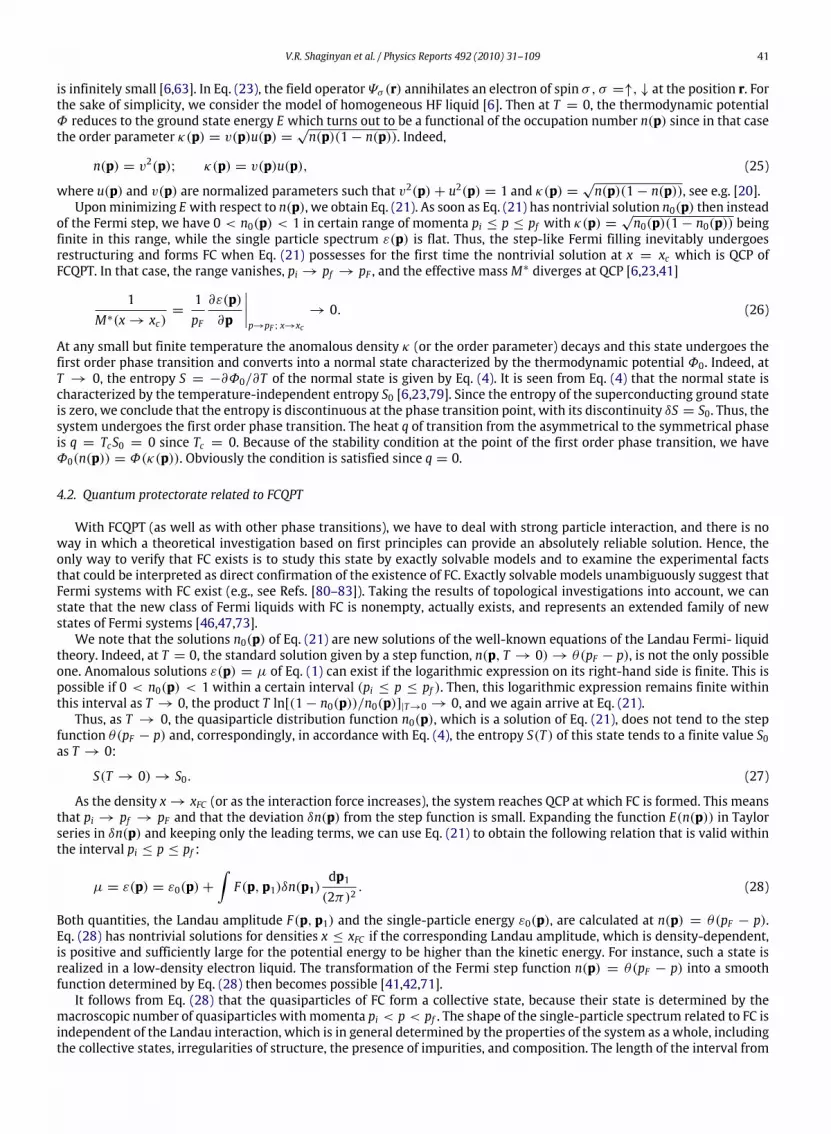
Fig. 5. The single-particle spectrum ε(p) and the quasiparticle distribution function n0(p). Because n0(p) is a solution of Eq. (21), we have n0(p < pi) = 1,0 < n0(pi < p < pf ) < 1, and n0(p > pf ) = 0, while ε(pi < p < pf ) = µ. The Fermi momentum pF satisfies the condition pi < pF < pf .
Fermi surface is proportional to the inverse effective mass, the potential energy of the quasiparticles near the Fermi surfacedetermines the ground-state energy as x→ xFC . Hence, a phase transition reduces the energy of the system and transformsthe quasiparticle distribution function. Beyond QCP x = xFC , the quasiparticle distribution is determined by the ordinaryequation for a minimum of the energy functional [41]:
δE(n(p))δn(p, T = 0)
= ε(p) = µ; pi ≤ p ≤ pf . (21)
Eq. (21) yields the quasiparticle distribution function n0(p) thatminimizes the ground-state energy E. This function foundfrom Eq. (21) differs from the step function in the interval from pi to pf , where 0 < n0(p) < 1, and coincides with the stepfunction outside this interval. In fact, Eq. (21) coincides with Eq. (3) provided that the Fermi surface at p = pF transformsinto the Fermi volume at pi ≤ p ≤ pf suggesting that the single-particle spectrum is absolutely ‘‘flat’’ within this interval. Apossible solution n0(p) of Eq. (21) and the corresponding single-particle spectrum ε(p) are depicted in Fig. 5. Quasiparticleswith momenta within the interval (pf − pi) have the same single-particle energies equal to the chemical potential µ andform FC, while the distribution n0(p) describes the new state of the Fermi liquid with FC [41,42,73]. In contrast to theLandau, marginal, or Luttinger–Fermi liquids [2,76,77], which exhibit the same topological structure of the Green’s function,in systemswith FC, where the Fermi surface spreads into a strip, the Green’s function belongs to a different topological class.The topological class of the Fermi liquid is characterized by the invariant [46,47,73]
N = tr∮C
dl2π iG(iω, p)∂lG−1(iω, p), (22)
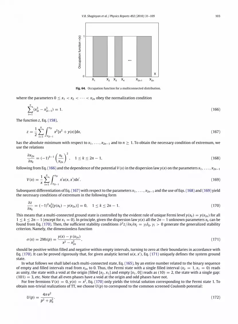
where ‘‘tr’’ denotes the trace over the spin indices of the Green’s function and the integral is taken along an arbitrary contourC encircling the singularity of the Green’s function. The invariant N in (22) takes integer values even when the singularityis not of the pole type, cannot vary continuously, and is conserved in a transition from the Landau Fermi liquid to marginalliquids and under small perturbations of the Green’s function. As shown by Volovik [46,47,73], the situation is quite differentfor systems with FC, where the invariant N becomes a half-integer and the system with FC transforms into an entirely newclass of Fermi liquids with its own topological structure.
4.1. The order parameter of FCQPT
We start with visualizing the main properties of FCQPT. To this end, again consider SCDFT. SCDFT states that thethermodynamic potential Φ is a universal functional of the number density n(r) and the anomalous density (or theorder parameter) κ(r, r1), providing a variational principle to determine the densities. At the superconducting transitiontemperature Tc a superconducting state undergoes the second order phase transition. Our goal now is to construct a quantumphase transition which evolves from the superconducting one.Let us assume that the coupling constant λ0 of the BCS-like pairing interaction [78] vanishes, with λ0 → 0making vanish
the superconducting gap at any finite temperature. In that case, Tc → 0 and the superconducting state takes place at T = 0while at finite temperatures there is a normal state. This means that at T = 0 the anomalous density
is infinitely small [6,63]. In Eq. (23), the field operatorΨσ (r) annihilates an electron of spin σ , σ =↑,↓ at the position r. Forthe sake of simplicity, we consider the model of homogeneous HF liquid [6]. Then at T = 0, the thermodynamic potentialΦ reduces to the ground state energy E which turns out to be a functional of the occupation number n(p) since in that casethe order parameter κ(p) = v(p)u(p) =
√n(p)(1− n(p)). Indeed,
n(p) = v2(p); κ(p) = v(p)u(p), (25)
where u(p) and v(p) are normalized parameters such that v2(p)+ u2(p) = 1 and κ(p) =√n(p)(1− n(p)), see e.g. [20].
Uponminimizing E with respect to n(p), we obtain Eq. (21). As soon as Eq. (21) has nontrivial solution n0(p) then insteadof the Fermi step, we have 0 < n0(p) < 1 in certain range of momenta pi ≤ p ≤ pf with κ(p) =
√n0(p)(1− n0(p)) being
finite in this range, while the single particle spectrum ε(p) is flat. Thus, the step-like Fermi filling inevitably undergoesrestructuring and forms FC when Eq. (21) possesses for the first time the nontrivial solution at x = xc which is QCP ofFCQPT. In that case, the range vanishes, pi → pf → pF , and the effective massM∗ diverges at QCP [6,23,41]
1M∗(x→ xc)
=1pF
∂ε(p)∂p
∣∣∣∣p→pF ; x→xc
→ 0. (26)
At any small but finite temperature the anomalous density κ (or the order parameter) decays and this state undergoes thefirst order phase transition and converts into a normal state characterized by the thermodynamic potential Φ0. Indeed, atT → 0, the entropy S = −∂Φ0/∂T of the normal state is given by Eq. (4). It is seen from Eq. (4) that the normal state ischaracterized by the temperature-independent entropy S0 [6,23,79]. Since the entropy of the superconducting ground stateis zero, we conclude that the entropy is discontinuous at the phase transition point, with its discontinuity δS = S0. Thus, thesystem undergoes the first order phase transition. The heat q of transition from the asymmetrical to the symmetrical phaseis q = TcS0 = 0 since Tc = 0. Because of the stability condition at the point of the first order phase transition, we haveΦ0(n(p)) = Φ(κ(p)). Obviously the condition is satisfied since q = 0.
4.2. Quantum protectorate related to FCQPT
With FCQPT (as well as with other phase transitions), we have to deal with strong particle interaction, and there is noway in which a theoretical investigation based on first principles can provide an absolutely reliable solution. Hence, theonly way to verify that FC exists is to study this state by exactly solvable models and to examine the experimental factsthat could be interpreted as direct confirmation of the existence of FC. Exactly solvable models unambiguously suggest thatFermi systems with FC exist (e.g., see Refs. [80–83]). Taking the results of topological investigations into account, we canstate that the new class of Fermi liquids with FC is nonempty, actually exists, and represents an extended family of newstates of Fermi systems [46,47,73].We note that the solutions n0(p) of Eq. (21) are new solutions of the well-known equations of the Landau Fermi- liquid
theory. Indeed, at T = 0, the standard solution given by a step function, n(p, T → 0)→ θ(pF − p), is not the only possibleone. Anomalous solutions ε(p) = µ of Eq. (1) can exist if the logarithmic expression on its right-hand side is finite. This ispossible if 0 < n0(p) < 1 within a certain interval (pi ≤ p ≤ pf ). Then, this logarithmic expression remains finite withinthis interval as T → 0, the product T ln[(1− n0(p))/n0(p)]|T→0 → 0, and we again arrive at Eq. (21).Thus, as T → 0, the quasiparticle distribution function n0(p), which is a solution of Eq. (21), does not tend to the step
function θ(pF − p) and, correspondingly, in accordance with Eq. (4), the entropy S(T ) of this state tends to a finite value S0as T → 0:
S(T → 0)→ S0. (27)
As the density x→ xFC (or as the interaction force increases), the system reaches QCP at which FC is formed. This meansthat pi → pf → pF and that the deviation δn(p) from the step function is small. Expanding the function E(n(p)) in Taylorseries in δn(p) and keeping only the leading terms, we can use Eq. (21) to obtain the following relation that is valid withinthe interval pi ≤ p ≤ pf :
µ = ε(p) = ε0(p)+∫F(p, p1)δn(p1)
dp1(2π)2
. (28)
Both quantities, the Landau amplitude F(p, p1) and the single-particle energy ε0(p), are calculated at n(p) = θ(pF − p).Eq. (28) has nontrivial solutions for densities x ≤ xFC if the corresponding Landau amplitude, which is density-dependent,is positive and sufficiently large for the potential energy to be higher than the kinetic energy. For instance, such a state isrealized in a low-density electron liquid. The transformation of the Fermi step function n(p) = θ(pF − p) into a smoothfunction determined by Eq. (28) then becomes possible [41,42,71].It follows from Eq. (28) that the quasiparticles of FC form a collective state, because their state is determined by the
macroscopic number of quasiparticles with momenta pi < p < pf . The shape of the single-particle spectrum related to FC isindependent of the Landau interaction, which is in general determined by the properties of the system as a whole, includingthe collective states, irregularities of structure, the presence of impurities, and composition. The length of the interval from
pi to pf where FC exists is the only characteristic determined by the Landau interaction; of course, the interaction must bestrong enough for FCQPT to occur. Therefore, we conclude that spectra related to FC have a universal shape. In Sections 4.3and5.1we show that these spectra are dependent on the temperature and the superconducting gap and that this dependenceis also universal. The existence of such spectra can be considered a characteristic feature of a ‘‘quantum protectorate’’, inwhich the properties of the material, including the thermodynamic properties, are determined by a certain fundamentalprinciple [84,85]. In our case, the state of matter with FC is also a quantum protectorate, since the new type of quasiparticlesof this state determines the special universal thermodynamic and transport properties of Fermi liquids with FC.
4.3. The influence of FCQPT at finite temperatures
According to Eq. (1), the single-particle energy ε(p, T ) is linear in T for T Tf within the interval (pf−pi) [86]. Expandingln((1− n(p))/n(p)) in a series in n(p) at p ' pF , we can write the expression
ε(p, T )− µ(T )T
= ln1− n(p)n(p)
'1− 2n(p)n(p)
∣∣∣∣p'pF
(29)
where Tf is the temperature above which the effect of FC is insignificant [51]:
TfεF∼p2f − p
2i
2MεF∼ΩFC
ΩF(30)
with ΩFC being the volume occupied by FC, εF being the Fermi energy, and ΩF being the volume of the Fermi sphere. Wenote that for T Tf , the occupation numbers n(p) obtained from Eq. (21) are almost perfectly independent of T [51,52,86].At finite temperatures, according to Eq. (29), the dispersionless plateau ε(p) = µ shown in Fig. 5 is slightly rotatedcounterclockwise in relation to µ. As a result, the plateau is slightly tilted and rounded off at its end points. Accordingto Eqs. (6) and (29), the effective massM∗FC that refers to the FC quasiparticles is given by
M∗FC ' pFpf − pi4T
. (31)
In deriving (31), we approximated the derivative as dn(p)/dp ' −1/(pf−pi). Eq. (31) clearly shows that for 0 < T Tf , theelectron liquid with FC behaves as if it were placed at a quantum critical point, since the electron effective mass diverges asT → 0. Actually, as we shall see in Section 4.4 the system is at a quantum critical line, because critical behavior is observedbehind QCP with x = xFC of FCQPT as T → 0. In Sections 7 and 10, we show that the behavior of such a system differsdramatically from that of a system at a quantum critical point.Upon using Eqs. (30) and (31), we estimate the effective massM∗FC as
M∗FCM∼N(0)N0(0)
∼TfT, (32)
where N0(0) is the density of states of a noninteracting electron gas and N(0) is the density of states on the Fermi surface.Eqs. (31) and (32) yield the temperature dependence ofM∗FC .Multiplying both sides of Eq. (31) by (pf − pi), we obtain an expression for the characteristic energy,
E0 ' 4T , (33)
which determines the momentum interval (pf − pi) with the low-energy quasiparticles characterized by the energy|ε(p) − µ| ≤ E0/2 and the effective mass M∗FC . The quasiparticles that do not belong to this momentum interval havean energy |ε(p) − µ| > E0/2 and an effective mass M∗L that is weakly temperature-dependent [74,75,87]. Eq. (33) showsthat E0 is independent of the condensate volume. We conclude from Eqs. (31) and (33) that for T Tf , the single-electronspectrum of FC quasiparticles has a universal shape and has the features of a quantum protectorate.Thus, a system with FC is characterized by two effective masses, M∗FC and M
∗
L . This fact manifests itself in a break or anabrupt change in the quasiparticle dispersion law, which for quasiparticles with energies ε(p) ≤ µ can be approximated bytwo straight lines intersecting at E0/2 ' 2T . Fig. 5 shows that at T = 0, the straight lines intersect at p = pi. This break alsooccurs when the system is in its superconducting state at temperatures Tc ≤ T Tf , where Tc is the critical temperature ofthe superconducting phase transition, which agrees with the experimental data in [88] and, as we will see in Section 5, thisbehavior agrees with the experimental data at T ≤ Tc . At T > Tc , the quasiparticles are well-defined, because their width γis small compared to their energy and is proportional to the temperature, γ ∼ T [34,51]. The quasiparticle excitation curve(see Section 6) can be approximately described by a simple Lorentzian [87], which also agrees with the experimental data[88–91].We estimate the density xFC at which FCQPT occurs. We show in Section 8 that an unlimited increase in the effective
mass precedes the appearance of a density wave or a charge density wave formed in electron systems at rs = rcdw , wherers = r0/aB, r0 is the average distance between electrons, and aB is the Bohr radius. Hence, FCQPT certainly occurs at T = 0
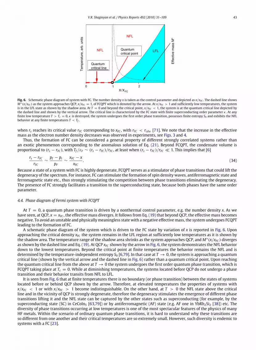
Fig. 6. Schematic phase diagram of system with FC. The number density x is taken as the control parameter and depicted as x/xFC . The dashed line showsM∗(x/xFC ) as the system approaches QCP, x/xFC = 1, of FCQPT which is denoted by the arrow. At x/xFC > 1 and sufficiently low temperatures, the systemis in the LFL state as shown by the shadow area. At T = 0 and beyond the critical point, x/xFC < 1, the system is at the quantum critical line depicted bythe dashed line and shown by the vertical arrow. The critical line is characterized by the FC state with finite superconducting order parameter κ . At anyfinite low temperature T > Tc = 0, κ is destroyed, the system undergoes the first order phase transition, possesses finite entropy S0 and exhibits the NFLbehavior at any finite temperatures T < Tf .
when rs reaches its critical value rFC corresponding to xFC , with rFC < rcdw [71]. We note that the increase in the effectivemass as the electron number density decreases was observed in experiments, see Figs. 3 and 4.Thus, the formation of FC can be considered a general property of different strongly correlated systems rather than
an exotic phenomenon corresponding to the anomalous solution of Eq. (21). Beyond FCQPT, the condensate volume isproportional to (rs − rFC ), with Tf /εF ∼ (rs − rFC )/rFC , at least when (rs − rFC )/rFC 1. This implies that [6]
rs − rFCrFC
∼pf − pipF
∼xFC − xxFC
. (34)
Because a state of a systemwith FC is highly degenerate, FCQPT serves as a stimulator of phase transitions that could lift thedegeneracy of the spectrum. For instance, FC can stimulate the formation of spin density waves, antiferromagnetic state andferromagnetic state etc., thus strongly stimulating the competition between phase transitions eliminating the degeneracy.The presence of FC strongly facilitates a transition to the superconducting state, because both phases have the same orderparameter.
4.4. Phase diagram of Fermi system with FCQPT
At T = 0, a quantum phase transition is driven by a nonthermal control parameter, e.g. the number density x. As wehave seen, at QCP, x = xFC , the effective mass diverges. It follows from Eq. (19) that beyond QCP, the effective mass becomesnegative. To avoid an unstable and physicallymeaningless statewith a negative effectivemass, the system undergoes FCQPTleading to the formation of FC.A schematic phase diagram of the system which is driven to the FC state by variation of x is reported in Fig. 6. Upon
approaching the critical density xFC the system remains in the LFL region at sufficiently low temperatures as it is shown bythe shadow area. The temperature range of the shadow area shrinks as the system approaches QCP, andM∗(x/xFC ) divergesas shown by the dashed line and Eq. (19). At QCP xFC shown by the arrow in Fig. 6, the system demonstrates the NFL behaviordown to the lowest temperatures. Beyond the critical point at finite temperatures the behavior remains the NFL and isdetermined by the temperature-independent entropy S0 [6,79]. In that case at T → 0, the system is approaching a quantumcritical line (shown by the vertical arrow and the dashed line in Fig. 6) rather than a quantum critical point. Upon reachingthe quantum critical line from the above at T → 0 the system undergoes the first order quantum phase transition, which isFCQPT taking place at Tc = 0. While at diminishing temperatures, the systems located before QCP do not undergo a phasetransition and their behavior transits from NFL to LFL.It is seen from Fig. 6 that at finite temperatures there is no boundary (or phase transition) between the states of systems
located before or behind QCP shown by the arrow. Therefore, at elevated temperatures the properties of systems withx/xFC < 1 or with x/xFC > 1 become indistinguishable. On the other hand, at T > 0 the NFL state above the criticalline and in the vicinity of QCP is strongly degenerate, therefore the degeneracy stimulates the emergence of different phasetransitions lifting it and the NFL state can be captured by the other states such as superconducting (for example, by thesuperconducting state (SC) in CeCoIn5 [63,79]) or by antiferromagnetic (AF) state (e.g. AF one in YbRh2Si2 [38]) etc. Thediversity of phase transitions occurring at low temperatures is one of the most spectacular features of the physics of manyHF metals. Within the scenario of ordinary quantum phase transitions, it is hard to understand why these transitions areso different from one another and their critical temperatures are so extremely small. However, such diversity is endemic tosystems with a FC [23].
Upon using nonthermal tuning parameters like the number density, pressure or magnetic field, the NFL behavior isdestroyed and the LFL one is restored as we shall see in Sections 9 and 10. For example, the application of magnetic fieldB > Bc0 drives a system to QCP and destroys the AF state restoring the LFL behavior. Here, Bc0 is a critical magnetic field,such that at B > Bc0 the system is driven towards its LFL state. In some cases as in the HF metal CeRu2Si2, Bc0 = 0, seee.g. [92], while in YbRh2Si2, Bc0 ' 0.06 T [15].
5. The superconducting state with FC
In this section we discuss the superconducting state of a 2D liquid of heavy electrons, since high-Tc superconductors arerepresented mainly by 2D structures. On the other hand, our study can easily be generalized to the 3D case. To show thatthere is no fundamental difference between the 2D and 3D cases, we derive Green’s functions for the 3D case in Section 5.2.
5.1. The superconducting state at T = 0
As we have seen in Section 4.1, the ground-state energy Egs(κ(p), n(p)) of a 2D electron liquid is a functional of thesuperconducting state order parameter κ(p) and of the quasiparticle occupation numbers n(p). This energy is determinedby the well-known Bardeen–Cooper–Schrieffer (BCS) equations and in the weak-coupling superconductivity theory is givenby [54,78,93]
It is assumed that the constant λ0, which determines the magnitude of the pairing interaction λ0V (p1, p2), is small. Wedefine the superconducting gap as
∆(p) = −λ0∫V (p, p1)κ(p1)
dp14π2
. (36)
Minimizing Egs in v(p) and using (36), we arrive at equations that relate the single-particle energy ε(p) to∆(p) and E(p)
ε(p)− µ = ∆(p)1− 2v2(p)2κ(p)
,∆(p)E(p)
= 2κ(p). (37)
Here the single-particle energy ε(p) is determined by Eq. (3), and
E(p) =√ξ 2(p)+∆2(p), (38)
with ξ(p) = ε(p)−µ. Substituting the expression for κ(p) from (37) in Eq. (36), we obtain the well-known equation of theBCS theory for∆(p)
∆(p) = −λ0
2
∫V (p, p1)
∆(p1)E(p1)
dp14π2
. (39)
As λ0 → 0, the maximum value of∆1 of the superconducting gap∆(p) tends to zero and each equation in (37) reduces toEq. (21)
δE(n(p))δn(p)
= ε(p)− µ = 0, (40)
if 0 < n(p) < 1, orκ(p) 6= 0, in the interval pi ≤ p ≤ pf . Eq. (40) shows that the function n0(p) is determined fromthe solution to the standard problem of finding the minimum of the functional E(n(p)) [41,51,52]. Eq. (40) specifies thequasiparticle distribution function n0(p) that ensures the minimum of the ground-state energy E(κ(p), n(p)). We can nowstudy the relation between the state specified by Eq. (40) or Eq. (21) and the superconducting state.At T = 0, Eq. (40) determines the specific state of a Fermi liquid with FC, the state for which the absolute value of
the order parameter |κ(p)| is finite in the momentum interval pi ≤ p ≤ pf as ∆1 → 0. Such a state can be consideredsuperconducting with an infinitely small value of ∆1. Hence, the entropy of this state at T = 0 is zero. Solutions n0(p) ofEq. (40) constitute a new class of solutions of both the BCS equations and the Landau Fermi-liquid equations. In contrast tothe ordinary solutions of the BCS equations [78], the new solutions are characterized by an infinitely small superconductinggap∆1 → 0, with the order parameter κ(p) remaining finite. On the other hand, in contrast to the standard solution of theLandau Fermi-liquid theory, the new solutions n0(p) determine the state of a heavy-electron liquid with a finite entropyS0 as T → 0 (see Eq. (27)). We arrive at an important conclusion that the solutions of Eq. (40) can be interpreted as thegeneral solutions of the BCS equations and the Landau Fermi-liquid theory equations, while Eq. (40) itself can be derivedeither from the BCS theory or from the Landau Fermi-liquid theory. Thus, as shown in Section 4.1 both states of the systemcoexist as T → 0. As the system passes into a state with the order parameter κ(p), the entropy suddenly vanishes, withthe system undergoing the first-order transition near which the critical quantum and thermal fluctuations are suppressed
and the quasiparticles are well- defined excitations (see also Section 10). It follows from Eq. (22) that FCQPT is related toa change in the topological structure of the Green’s function and belongs to Lifshitz’s topological phase transitions, whichoccur at absolute zero [73]. This fact establishes a relation between FCQPT and quantum phase transitions under which theFermi sphere splits into a sequence of Fermi layers [94,95] (see Sections 7 and 15). We note that in the state with the orderparameter κ(p), the system entropy S = 0 and the Nernst theorem holds in systems with FC.If λ0 6= 0, the gap ∆1 becomes finite, leading to a finite value of the effective mass M∗FC , which may be obtained from
Eq. (37) by taking the derivative with respect to the momentum p of both sides and using Eq. (6) [74,75,87]:
M∗FC ' pFpf − pi2∆1
. (41)
It follows from Eq. (41) that in the superconducting state the effective mass is always finite. As regards the energy scale, itis determined by the parameter E0:
E0 = ε(pf )− ε(pi) ' pF(pf − pi)M∗FC
' 2∆1. (42)
5.2. Green’s function of the superconducting state with FC at T = 0
We write two equations for the 3D case, the Gor’kov equations [96], which determine the Green’s functions F+(p, ω)and G(p, ω) of a superconductor (e.g., see Ref. [20]):
F+ =−λ0Ξ
∗
(ω − E(p)+ i0)(ω + E(p)− i0);
G =u2(p)
ω − E(p)+ i0+
v2(p)ω + E(p)− i0
(43)
The gap∆ and the functionΞ are given by
∆ = λ0|Ξ |, iΞ =∫ ∫
∞
−∞
F+(p, ω)dωdp(2π)4
. (44)
We recall that the function F+(p, ω) has the meaning of the wave function of Cooper pairs and Ξ is the wave function ofthe motion of these pairs as a whole and is just a constant in a homogeneous system [20]. It follows from Eqs. (37) and (44)that
iΞ =∫∞
−∞
F+0 (p, ω)dωdp(2π)4
= i∫κ(p)
dp(2π)3
. (45)
Taking Eqs. (44) and (37) into account, we can write Eq. (43) as
F+ = −κ(p)
ω − E(p)+ i0+
κ(p)ω + E(p)− i0
;
G =u2(p)
ω − E(p)+ i0+
v2(p)ω + E(p)− i0
. (46)
As λ0 → 0, the gap∆→ 0, butΞ and κ(p) remain finite if the spectrum becomes flat, E(p) = 0, and Eq. (46) become
F+(p, ω) = −κ(p)[
1ω + i0
−1
ω − i0
];
G(p, ω) =u2(p)ω + i0
+v2(p)ω − i0
(47)
in the interval pi ≤ p ≤ pf . The parameters v(p) and u(p) are determined by the condition that the spectrum be flat:ε(p) = µ. If we take the Landau equation (3) into account, this condition again reduces to Eq. (21) and (40) for determiningthe minimum of the functional E(n(p)).We construct the functions F+(p, ω) and G(p, ω) in the case where the constant λ0 is finite but small, such that v(p)
and κ(p) can be found on the basis of the FC solutions of Eq. (21). Then Ξ , E(p) and∆ are given by Eqs. (45), (44) and (37)respectively. Substituting the functions constructed in this manner into (46), we obtain F+(p, ω) and G(p, ω) [97]. We notethat Eq. (44) imply that the gap∆ is a linear function of λ0 under the adopted conditions. As we shall see in Section 5.3, thisgives rise to high-Tc at common values of the superconducting coupling constant.
5.3. The superconducting state at finite temperatures
We assume that the region occupied by FC is small: (pf − pi)/pF 1 and ∆1 Tf . Then, the order parameter κ(p) isdetermined primarily by FC, i.e., the distribution function n0(p) [74,75]. To be able to solve Eq. (39) analytically, we adoptthe BCS approximation for the interaction [78]: λ0V (p, p1) = −λ0 if |ε(p)−µ| ≤ ωD and the interaction is zero outside thisregion, withωD being a certain characteristic energy. As a result, the superconducting gap depends only on the temperature,∆(p) = ∆1(T ), and Eq. (39) becomes
1 = NFCλ0
∫ E0/2
0
dξ√ξ 2 +∆21(0)
+ NLλ0
∫ ωD
E0/2
dξ√ξ 2 +∆21(0)
(48)
where we introduced the notation ξ = ε(p) − µ and the density of states NFC in the interval (pf − pi) or in the E0-energyinterval. It follows from Eq. (41) that NFC = (pf − pF )pF/(2π∆1). Within the energy interval (ωD − E0/2), the density ofstates NL has the standard form NL = M∗L /2π . As E0 → 0, Eq. (48) becomes the BCS equation. On the other hand, assumingthat E0 ≤ 2ωD and discarding the second integral on the right-hand side of Eq. (48), we obtain
∆1(0) =λ0pF (pf − pF )
2πln(1+√2)
= 2βεFpf − pFpF
ln(1+√2), (49)
where εF = p2F/2M∗
L is the Fermi energy and β = λ0M∗L /2π is the dimensionless coupling constant. Using the standardvalue of β for ordinary superconductors, e.g., β ' 0.3, and assuming that (pf − pF )/pF ' 0.2, we obtain a large value∆1(0) ∼ 0.1εF from Eq. (49); for ordinary superconductors, this gap has a much smaller value: ∆1(0) ∼ 10−3εF . With theintegral discarded earlier taken into account, we find that
∆1(0) ' 2βεFpf − pFpF
ln(1+√2)+∆1(0)β ln
(2ωD∆1(0)
). (50)
On the right-hand side of Eq. (50), the value of∆1 is given by (49). As E0 → 0 and pf → pF , the first term on the right-handside of Eq. (48) is zero, and we obtain the ordinary BCS result with∆1 ∝ exp(−1/λ0). The correction related to the secondintegral in Eq. (48) is small because the second term on the right-hand side of Eq. (50) contains the additional factor β . Inwhat follows, we show that 2Tc ' ∆1(0). The isotopic effect is small in this case, because Tc depends on ωD logarithmical,but the effect is restored as E0 → 0.At T ' Tc , Eqs. (41) and (42) are replaced by Eqs. (31) and (33), which also hold for Tc ≤ T Tf :
M∗FC ' pFpf − pi4Tc
, E0 ' 4Tc, if T ' Tc; (51)
M∗FC ' pFpf − pi4T
, E0 ' 4T , at T < Tc . (52)
Eq. (48) is replaced by its standard generalization valid for finite temperatures:
1 = NFCλ0
∫ E0/2
0
dξ√ξ 2 +∆21
tanh
√ξ 2 +∆21
2T+ NLλ0
∫ ωD
E0/2
dξ√ξ 2 +∆21
tanh
√ξ 2 +∆21
2T. (53)
Because∆1(T → Tc)→ 0, Eq. (53) implies a relation that closely resembles the BCS result [5],
2Tc ' ∆1(0), (54)
where ∆1(T = 0) is found from Eq. (50). Comparing (41) and (42) with (51) and (52), we see that both M∗FC and E0 aretemperature-independent for T ≤ Tc .
5.4. Bogoliubov quasiparticles
Eq. (39) shows that the superconducting gap depends on the single-particle spectrum ε(p). On the other hand, it followsfrom Eq. (37) that ε(p) depends on ε(p) if Eq. (40) has a solution that determines the existence of FC as λ0 → 0. We assumethat λ0 is so small that the pairing interaction λ0V (p, p1) leads only to a small perturbation of the order parameter κ(p).Eq. (41) implies that the effective mass and the density of states N(0) ∝ M∗FC ∝ 1/∆1 are finite. Thus, in contrastto the spectrum in the standard superconductivity theory, the single-particle spectrum ε(p) depends strongly on thesuperconducting gap, and Eqs. (3) and (39) must be solved by a self-consistent method.
We assume that Eqs. (3) and (39) have been solved and the effective mass M∗FC has been found. This means that wecan find the quasiparticle dispersion law ε(p) by choosing the effective mass M∗ equal to the obtained value of M∗FCand then solve Eq. (39) without taking (3) into account, as is done in the standard BCS superconductivity theory [78].Hence, the superconducting state with FC is characterized by Bogoliubov quasiparticles [98] with dispersion (38) and thenormalization condition v2(p) + u2(p) = 1 for the coefficients v(p) and u(p). Moreover, quasiparticle excitations of thesuperconducting state in the presence of FC coincidewith the Bogoliubov quasiparticles characteristic of the BCS theory, andsuperconductivity with FC resembling the BCS superconductivity, which points to the applicability of the BCS formalism tothe description of the high-Tc superconducting state [99]. At the same time, themaximum value of the superconducting gapset by Eq. (50) and other exotic properties are determined by the presence of FC. These results are in good agreement withthe experimental facts obtained for the high-Tc superconductor Bi2Sr2Ca2Cu3O10+δ [100].In constructing the superconducting statewith FC,we returned to the foundations of the LFL theory, fromwhich the high-
energy degrees of freedom had been eliminated by the introduction of quasiparticles. The main difference between the LFL,which forms the basis for constructing the superconducting state, and the Fermi liquid with FC is that in the latter case wemust increase the number of low-energy degrees of freedom by introducing the new type of quasiparticle with the effectivemass M∗FC and the characteristic energy E0 given by Eq. (42). Hence, the dispersion law ε(p) is characterized by two typesof quasiparticles with the effective masses M∗L and M
∗
FC and the scale E0. The extended paradigm and new quasiparticlesdetermine the properties of the superconductor, including the lineshape of quasiparticle excitations [74,75,101], while thedispersion of the Bogoliubov quasiparticles has the standard form.We note that for T < Tc , the effective mass M∗FC and the scale E0 are temperature-independent [101]. For T > Tc ,
the effective mass M∗FC and the scale E0 are given by Eqs. (31) and (33). Obviously, we cannot directly relate these newquasiparticles (excitations) of the Fermi liquid with FC to excitations (quasiparticles) of an ideal Fermi gas, as is done in thestandard LFL theory, because the system is beyond FCQPT. The properties and dynamics of quasiparticles are given by theextended paradigm and closely related to the properties of the superconducting state and are of a collective nature, formedby FCQPT and determined by the macroscopic number of FC quasiparticles with momenta in the interval (pf − pi). Such asystem cannot be perturbed by scattering on impurities and lattice defects and, therefore, has the features of a quantumprotectorate and demonstrates universal behavior [74,75,84,85].Several remarks concerning the quantum protectorate and the universal behavior of superconductors with FC are in
order. Similarly to the Landau Fermi liquid theory, the theory of high-Tc superconductivity based on FCQPT deals withquasiparticles that are elementary low-energy excitations. The theory provides a qualitative general description of thesuperconducting and the normal states of superconductors and HF metals. Of course, with phenomenological parameters(e.g., the pairing coupling constant) chosen, we can obtain a quantitative description of superconductivity, in the same wayas this can be done in the Landau theory when describing a normal Fermi liquid, e.g., 3He. Hence, any theory capable ofdescribing FC and compatible with the BCS theory gives the same qualitative picture of the superconducting and normalstates as the picture based on FCQPT. Obviously, both approaches may be coordinated on the level of numerical resultsby choosing the appropriate parameters. For instance, because the formation of FC is possible in the Hubbard model [83], itallows reproducing the results of the theory based on FCQPT. It is appropriate to note here that the corresponding descriptionrestricted to the case of T = 0 has been obtained within the framework of the Hubbard model [102,103].
5.5. The pseudogap
We now discuss some features of the superconducting state with FC [57,87,104] considering two possible types of thesuperconducting gap∆(p) determined by Eq. (39) and the interaction λ0V (p, p1). If the interaction is caused by attraction,occurring, for instance, as a result of an exchange of phonons ormagnetic excitations, the solution of Eq. (39) with an s-waveor s+d-mixedwaves has the lowest energy. If the pairing interactionλ0V (p1, p2) is a combination of an attractive interactionand a strongly repulsive interaction, d-wave superconductivity may occur (e.g., see Refs. [105,106]). However, both thes- and d-wave symmetries lead to approximately the same result for the size of the gap ∆1 in Eq. (50). Hence, d-wavesuperconductivity is not a universal and necessary property of high-Tc superconductors. This conclusion agrees with theexperimental evidence described in Refs. [107–111].We can define the critical temperature T ∗ as the temperature at which ∆1(T ∗) ≡ 0. For T ≥ T ∗, Eq. (53) has
only the trivial solution ∆1 ≡ 0. On the other hand, the critical temperature Tc can be defined as the temperature atwhich superconductivity disappears and the gap occupies only a part of the Fermi surface. Thus, there are two differenttemperatures Tc and T ∗, which may not coincide in the case of the d-wave symmetry of the gap. As shown in Refs. [57,87],in the presence of FC, Eq. (53) has nontrivial solutions at Tc ≤ T ≤ T ∗, when the pairing interaction λ0V (p1, p2) consistsof attraction and strong repulsion, which leads to d-wave superconductivity. In this case, the gap ∆(p) as a function of theangle φ, or∆(p) = ∆(pF , φ), has new nodes at T > Tnode, as shown in Fig. 7 [87].Fig. 7 shows the ratio∆(pF , φ)/T ∗ calculated for three temperatures: 0.9 Tnode, Tnode and 1.2 Tnode. In contrast to curve (a),
curves (b) and (c) have flat sections. Clearly, the flattening occurs because of the two new zeros that emerge at T = Tnode. Asthe temperature increases, the region θc between the zeros (indicated by arrows in Fig. 7) increases in size. It is also clearthat the gap∆ is very small within the interval θc . It was found in [112,113] that the magnetism and the superconductivityaffect each other, which leads to suppression of the magnetism at temperatures below Tc . In view of this, we can expectsuppression of superconductivity due to magnetism.
Fig. 7. The gap ∆(pF , φ) as a function of φ calculated for three values of the temperature expressed in units of Tnode ' Tc . The solid curve (a) representsthe function ∆(pF , φ) calculated for the temperature 0.9 Tnode . The dashed curves (b) represents the same function at T = Tnode , and the dotted curve (c)depicts the function calculated at 1.2 Tnode . The arrows indicate the region θc limited by the two new zeros that emerge at T > Tnode .
0.7
0.6
0.5
0.4
0.3
0.2
0.1
0.00.00 0.05 0.10 0.15 0.20 0.25
Fig. 8. The result of a numerical calculation of the angle θc separating two zeros as a function of (T − Tc)/Tc .
Thus, we may conclude that the gap in the vicinity of Tc can be destroyed by strong antiferromagnetic correlations(or spin density waves), impurities, and sizable inhomogeneities existing in high-Tc superconductors [114]. Because thesuperconducting gap is destroyed in a macroscopic region of the phase space, θc , superconductivity is also destroyed, andtherefore Tc ' Tnode. The exact value of Tc is determined by the competition between the antiferromagnetic state (or spindensity waves) and the superconductivity in the interval θc . The behavior and the shape of the pseudogap closely resemblethe similar characteristics of the superconducting gap, as Fig. 7 shows. Themain difference is that the pseudogap disappearsin the segment θc of the Fermi surface, while the gap disappears at isolated nodes of the d-wave. This result is in accordwith observations [115]. Our estimates show that for small values of the angle ψ , the function θc(ψ) rapidly increases,θc(ψ) '
√ψ . These estimates agree with the results of numerical calculations of the function θc([T − Tc]/Tc), (Fig. 8).
Hence, we may conclude that Tc is close to Tnode. Thus, the pseudogap state appears at T ≥ Tc ' Tnode and disappears attemperatures T ≥ T ∗ at which Eq. (53) has only the trivial solution ∆1 ≡ 0. Obviously, ∆1 determines T ∗ and not Tc , withthe result that Eq. (54) should be rewritten as
2T ∗ ' ∆1(0). (55)
The temperature T ∗ has the physical meaning of the temperature of the BCS transition between the state with the orderparameter κ 6= 0 and the normal state.At temperatures below T < Tc , the quasiparticle excitations of the superconducting state are characterized by the
presence of sharp peaks.When the temperature becomes high (T > Tc) and∆(θ) ≡ 0 in the interval θc , normal quasiparticleexcitations with a width γ appear in the segments θc of the Fermi surface. A pseudogap exists outside the segments θc , andthe Fermi surface is occupied by excitations of the BCS type in this region. Excitations of both types have widths of the sameorder of magnitude, transferring their energy and momenta into excitations of normal quasiparticles. These results are inaccord with strong indications of the pairing or the formation of preformed pairs in the pseudogap regime at temperaturesabove Tc [115–120].
We now estimate the value of γ . If the entire Fermi surface were occupied by the normal state, the width γ would beγ ≈ N(0)3T 2/εd(T )2 with the density of states N(0) ∼ M∗(T ) ∼ 1/T [see Eq. (31)]. The dielectric constant εd(T ) ∼ N(0)and, hence, γ ∼ T [51,52]. However, only a part of the Fermi surface within θc is occupied by normal excitations in ourcase. Therefore, the number of states accessible for quasiparticles and quasiholes is proportional to θc , and the factor T 2 isreplaced by the factor T 2θ2c . Taking all this into account yields γ ∼ θ
2c T ∼ T (T − Tc)/Tc ∼ (T − Tc). Here, we ignored the
small contribution provided by excitations of the BCS type. It is precisely for this reason that the width γ vanishes at T = Tc .Moreover, the resistivity of the normal state ρ(T ) ∝ γ ∝ (T − Tc), because γ ∼ (T − Tc). Obviously, at temperaturesT > T ∗, the relation ρ(T ) ∝ γ ∝ T remains valid up to T ∼ Tf , and Tf may be as high as the Fermi energy if FC occupies asignificant part of the Fermi volume.The temperature Tnode is determined mainly by the repulsive interaction, which is part of the pairing interaction
λ0V (p1, p2). The value of the repulsive interaction, in turn, may be determined by the properties of the materials, suchas composition or doping. Because superconductivity is destroyed at Tc ' Tnode, the ratio 2∆1/Tc may vary within broadlimits and strongly depends on the properties of the material [57,87,104]. For instance, in the case of Bi2Sr2CaCu2O6+δ it isassumed that superconductivity and the pseudogap are of common origin: 2∆1/Tc ' 28, while 2∆1/T ∗ ' 4, which agreeswith the experimental data obtained in measurements involving other high-Tc superconductors [105].We note that Eq. (55) also provides a good description of the maximum value of the gap ∆1 in the case of d-wave
superconductivity, because different regions with the maximum density of states may be considered unrelated [106]. Wemay also conclude that without a strong repulsion, with which s-wave pairing is possible, there can be no pseudogap.Thus, the transition from the superconducting gap to the pseudogap may proceed only in the case of d-wave pairing, whensuperconductivity is destroyed at Tc ' Tnode and the superconducting gap gradually transforms into a pseudogap, whichcloses at a certain temperature T ∗ > Tc [57,87,104]. The fact that there is no pseudogap in the case of s-wave pairing agreeswith the experimental data (e.g., see Ref. [111]).
5.6. Dependence of the critical temperature Tc of the superconducting phase transition on doping
We examine the maximum value of the superconducting gap∆1 as a function of the number density x of mobile chargecarriers, which is proportional to the degree of doping. Using Eq. (34), we can rewrite Eq. (49) as
∆1
εF∼ β
(xFC − x)xxFC
(56)
where we took into account that the Fermi level εF ∝ p2F and that the number density x ∼ p2F/(2M
∗), with the resultthat εF ∝ x. It is realistic to assume that Tc ∝ ∆1, because the curve Tc(x) obtained in experiments with high-Tcsuperconductors [2] must be a smooth function of x. Hence, we can approximate Tc(x) by a smooth bell-shape function[121]:
Tc(x) ∝ β(xFC − x)x. (57)
To illustrate the application of the above analysis, we examine the main features of a superconductor that canhypothetically exist at room temperature. Such a superconductor must be a two-dimensional structure, just as high-Tcsuperconducting cuprates are. Eq. (49) implies that∆1 ∼ βεF ∝ β/r2s . Bearing in mind that FCQPT occurs at rs ∼ 20 in 3Dsystems and at rs ∼ 8 in 2D systems [71], we can expect that in 3D systems∆1 amounts to 10% of the maximum size of thesuperconducting gap in 2D systems, which in our case amounts to 60 mV for lightly doped cuprates with Tc = 70 K [122].On the other hand, Eq. (49) implies that∆1 may be even larger,∆1 ∼ 75 mV. We can expect that Tc ∼ 300 K in the case ofs-wave pairing, as the simple relation 2Tc ' ∆1 implies. Indeed, we can take εF ∼ 500mV, β ∼ 0.3, and (pf −pi)/pF ∼ 0.5.Thus, the hypothetical superconductor at room temperaturemust be an s-wave superconductor in order to eliminate the
pseudogap effect, which dramatically decreases the temperature Tc at which superconductivity is destroyed. We note thatthe number density x of mobile charge carriers must satisfy the condition x ≤ xFC and must be varied to reach the optimumdegree of doping xopt ' xFC/2.
5.7. The gap and heat capacity near Tc
We now calculate the gap and heat capacity at temperatures T → Tc . Our analysis is valid if T ∗ ' Tc , since otherwisethe discontinuities in the heat capacity considered below are smeared over the temperature interval between T ∗ and Tc . Tosimplify matters, we calculate the leading contribution to the gap and heat capacity related to FC. We use Eq. (53) to findthe function ∆1(T → Tc) simply by expanding the first integral on its right-hand side in powers of ∆1 and dropping thecontribution from the second integral. This procedure leads to the equation [101]
∆1(T ) ' 3.4Tc
√1−
TTc. (58)
Therefore, the gap in the spectrum of single-particle excitations behaves in the ordinary manner.
To calculate the heat capacity, we can use the standard expression for the entropy S [78]:
S(T ) = −2∫[f (p) ln f (p)+ (1− f (p)) ln(1− f (p))]
dp(2π)2
, (59)
where
f (p) = (1+ exp[E(p)/T ])−1,
E(p) =√(ε(p)− µ)2 +∆21(T ). (60)
The heat capacity C is given by
C(T ) = TdSdT' 4
NFCT 2
∫ E0
0f (E)(1− f (E))
[E2 + T∆1(T )
d∆1(T )dT
]dξ + 4
NLT 2
∫ ωD
E0f (E)(1− f (E))
×
[E2 + T∆1(T )
d∆1(T )dT
]dξ . (61)
In deriving Eq. (61), we again used the variable ξ , the above notation for the density of states, NFC and NL, and the notation
E =√ξ 2 +∆21(T ). Eq. (61) describes a jump in heat capacity, δC(T ) = Cs(T )−Cn(T ), where Cs(T ) and Cn(T ) are respectively
the heat capacities of the superconducting andnormal states at Tc ; the jump is determined by the last two terms in the squarebrackets on the right-hand side of this equation. Using Eq. (58) to calculate the first term on the right-hand side of Eq. (61),we find [101]
δC(Tc) '32π2
(pf − pi)pnF (62)
where n = 1 in the 2D case and n = 2 in the 3D case. This result differs from the ordinary BCS result, according to which thediscontinuity in the heat capacity is a linear function of Tc . The jump δC(Tc) is independent of Tc because, as Eq. (52) shows,the density of state varies in inverse proportion to Tc . We note that in deriving Eq. (62) we took the leading contributioncoming from FC into account. This contribution disappears as E0 → 0, and the second integral on the right-hand side ofEq. (61) yields the standard result.As we will show in Section 10 [see Eq. (134)], the heat capacity of a systemwith FC behaves as Cn(T ) ∝
√T/Tf . The jump
in the heat capacity given by Eq. (62) is temperature-independent. As a result, we find that
δC(Tc)Cn(Tc)
∼
√TfTc
(pf − pi)pF
. (63)
In contrast to the case of normal superconductors, in which δC(Tc)/Cn(Tc) = 1.43 [20], in our case Eq. (63) implies that theratio δC(Tc)/Cn(Tc) is not constant and may be very large when Tf /Tc 1 [79,101]. It is instructive to apply this analysis toCeCoIn5, where Tc = 2.3 K [79]. In this material [123], δC/Cn ' 4.5 is substantially higher than the BCS value, in agreementwith Eq. (63).
6. The dispersion law and lineshape of single-particle excitations
The recently discovered break in the dispersion of quasiparticles at energies between 40 and 70mV, resulting in a changein the quasiparticle speed at this energy [88–91], can hardly be explained by the marginal Fermi-liquid theory, becausethis theory contains no additional energy scales or parameters that would allow taking the break into account [76,77]. Wecould assume that the break, which leads to a new energy scale, occurs because of the interaction of electrons and collectiveexcitations, but thenwewould have to discard the idea of a quantumprotectorate, whichwould contradict the experimentaldata [84,85].As shown in Sections 4 and 5, a system with FC has two effective masses: M∗FC , which determines the single-particle
spectrum at low energies, and M∗L , which determines the spectrum at high energies. The fact that there are two effectivemasses manifests itself in the form of a break in the quasiparticle dispersion law. The dispersion law can be approximatedby two straight lines intersecting at a binding energy E0/2 [see Eqs. (33) and (42)]. The break in the dispersion law occursat temperatures much lower than T Tf , when the system is in the superconducting or normal state. Such behavior is ingood agreement with the experimental data [88]. It is pertinent to note that at temperatures below T < Tc , the effectivemassM∗FC is independent of the momenta pF , pf , and pi, as shown by Eqs. (41) and (49):
M∗FC ∼2πλ0. (64)
This formula implies that M∗FC is only weakly dependent on x if a dependence of λ0 on x is allowed. This result is in goodagreement with the experimental facts [124–126]. The same is true of the dependence of the Fermi velocity vF = pF/M∗FC
on x because the Fermi momentum pF ∼√n is weakly dependent on the electron number density n = n0(1− x) [124,125];
here, n0 is the single-particle electron number density at half-filling.Because λ0 is the coupling constant that determines the magnitude of the pairing interaction, e.g., the electron–phonon
interaction, we can expect the break in the quasiparticle dispersion law to be caused by the electron–phonon interaction.The phonon scenario could explain the constancy of the break at T > Tc because phonons are temperature independent.On the other hand, it was found that the quasiparticle dispersion law distorted by the interaction with phonons has atendency to restore itself to the ordinary single particle dispersion law when the quasiparticle energy becomes higher thanthe phonon energy [127]. However, there is no experimental evidence that such restoration of the dispersion law actuallytakes place [88].The quasiparticle excitation curve L(q, ω) is a function of two variables. Measurements at a constant energy ω = ω0,
where ω0 is the single particle excitation energy, determine the curve L(q, ω = ω0) as a function of the momentum q. Weestablished above that M∗FC is finite and constant at temperatures not exceeding Tc . Hence, at excitation energies ω < E0,the system behaves as an ordinary superconducting Fermi liquid with the effective mass determined by Eq. (41) [74,75,87].At Tc ≤ T , the effective mass M∗FC is also finite and is given by Eq. (31). In other words, at ω < E0, the system behaves as aFermi liquid whose single-particle spectrum is well defined and the width of the single-particle excitations is of the orderof T [74,75,51]. Such behavior has been observed in experiments in measuring the quasiparticle excitation curve at a fixedenergy [34,90,128].The quasiparticle excitation curve can also be described as a function of ω, at a constant momentum q = q0. For small
values of ω, the behavior of this function is similar to that described above, with L(q = q0, ω) having a characteristicmaximum and width. For ω ≥ E0, the contribution provided by quasiparticles of mass M∗L becomes significant and leadsto an increase in the function L(q = q0, ω). Thus, L(q = q0, ω) has a certain structure of maxima and minima [129]directly determined by the existence of two effectivemasses,M∗FC andM
∗
L [74,75,87].We conclude that, in contrast to Landauquasiparticles, these quasiparticles have a more complicated spectral lineshape.We use the Kramers–Kronig transformation to calculate the imaginary part ImΣ(p, ε) of the self-energy part Σ(p, ε).
But we begin with the real part ReΣ(p, ε), which determines the effective massM∗ [130],
1M∗=
(1m+1pF
∂ReΣ∂p
)/(1−
∂ReΣ∂ε
). (65)
The corresponding momenta p and energies ε satisfy the inequalities |p − pF |/pF 1, and ε/εF 1. We take ReΣ(p, ε)in the simplest form possible that ensures the variation of the effective mass at the energy E0/2,
ReΣ(p, ε) = −εM∗FCm+
(ε −
E02
)M∗FC −M
∗
L
m
[θ
(ε −
E02
)+ θ
(−ε −
E02
)], (66)
where θ(ε) is the step function. To ensure a smooth transition from the single-particle spectrum characterized by M∗FC tothe spectrum characterized by M∗L , we must replace the step function with a smoother function. Substituting Eq. (66) inEq. (65), we see that M∗ ' M∗FC within the interval (−E0/2, E0/2), while M
∗' M∗L outside this interval. Applying the
Kramers–Kronig transformation to ReΣ(p, ε), we express the imaginary part of the self-energy as [101]
ImΣ(p, ε) ∼ ε2M∗FCεFm+M∗FC −M
∗
L
m
[ε ln
∣∣∣∣2ε + E02ε − E0
∣∣∣∣+ E02 ln∣∣∣∣4ε2 − E20E20
∣∣∣∣] . (67)
Clearly, with ε/E0 1, the imaginary part is proportional to ε2; at 2ε/E0 ' 1, we have ImΣ ∼ ε, and for E0/ε 1, themain contribution to the imaginary part is approximately constant.It follows from Eq. (67) that as E0 → 0, the second term on its right-hand side tends to zero and the single-particle
excitations become well-defined, which resembles the situation with a normal Fermi liquid, while the pattern of minimaand maxima eventually disappears. Now the quasiparticle renormalization factor z(p) is given by the equation [130]
1z(p)= 1−
∂ReΣ(p, ε)∂ε
. (68)
Consequently, from Eqs. (67) and (68) for T ≤ Tc , the amplitude of a quasiparticle on the Fermi surface increases as thecharacteristic energy E0 decreases. Equations Eqs. (42) and (57) imply that E0 ∼ (xFC − x)/xFC . When T > Tc , it followsfrom (66) and (68) that the quasiparticle amplitude increases as the effective mass M∗FC decreases. So, from Eqs. (31) and(34) M∗FC ∼ (pf − pi)/pF ∼ (xFC − x)/xFC . As a result, we conclude that the amplitude increases with the doping level andthe single-particle excitations are better defined in heavily doped samples. As x → xFC , the characteristic energy E0 → 0and the quasiparticles become normal excitations of LFL. We note that such behavior has been observed in experimentswith heavily doped Bi2212, which demonstrates high-Tc superconductivity with a gap of about 10 mV [131]. The size of thegap suggests that the region occupied by FC is small because E0/2 ' ∆1. For x > xFC and low temperatures, the HF liquidbehaves as LFL (see Fig. 6 and Section 9). Experimental data show that, as expected, the LFL state exists in super-heavilydoped nonsuperconducting La1.7Sr0.3CuO4 [132,133].
Fig. 9. The function ν(p) for the multiply connected distribution that replaces the function n0(p) in the region (pf − pi) occupied by FC. The momentasatisfy the inequalities pi < pF < pf . The outer Fermi surface at p ' p2n ' pf has the shape of a Fermi step, and therefore the system behaves like LFL atsufficiently low temperatures.
7. Electron liquid with FC in magnetic fields
In this section, we discuss the behavior of HF liquid with FC in magnetic field. We assume that the coupling constant isnonzero, λ0 6= 0, but is infinitely small. We found in Section 5 that at T = 0 the superconducting order parameter κ(p)is finite in the region occupied by FC and that the maximum value of the superconducting gap ∆1 ∝ λ0 is infinitely small.Hence, any weak magnetic field B 6= 0 is critical and destroys κ(p) and FC. Simple energy arguments suffice to determinethe type of rearrangement of the FC state. On the one hand, because the FC state is destroyed, the gain in energy∆EB ∝ B2tends to zero as B→ 0. On the other hand, the function n0(p), which occupies the finite interval (pf −pi) in the momentumspace and is specified by Eq. (21) or (42), leads to a finite gain in the ground-state energy compared to the ground-stateenergy of a normal Fermi liquid [41]. Thus, the distribution function is to be reconstructed so that the order parameter is tovanish while a new distribution function is to deliver the same ground state energy.
7.1. Phase diagram of electron liquid in magnetic field
Thus, in weak magnetic fields, the new ground state without FC must have almost the same energy as the state with FC.As shown in Section 15, such a state is formed bymultiply connected Fermi spheres resembling an onion, in which a smoothdistribution function of quasiparticles, n0(p), is replaced in the interval (pf − pi)with the distribution function [94,134]
ν(p) =n∑k=1
θ(p− p2k−1)θ(p2k − p) (69)
where the parameters pi ≤ p1 < p2 < · · · < p2n ≤ pf are chosen such that they satisfy the normalization condition andthe condition needed for the conservation of the number of particles:∫ p2k+3
p2k−1ν(p)
dp(2π)3
=
∫ p2k+3
p2k−1n0(p)
dp(2π)3
.
Fig. 9 shows the corresponding multiply connected distribution. For definiteness, we present the most interesting caseof a three-dimensional system. The two-dimensional case can be examined similarly. We note that the possibility of theexistence of multiply connected Fermi spheres was studied in e.g. [23,135–137].We assume that the thickness of each inner slice of the Fermi sphere, δp ' p2k+1−p2k, is determined by themagnetic field
B. Using the well-known rule for estimating errors in calculating integrals, we find that the minimum loss of the ground-state energy due to slice formation is approximately (δp)4. This becomes especially clear if we account for the fact thatthe continuous FC functions n0(p) ensure the minimum value of the energy functional E[n(p)], while the approximation ofν(p) by steps of width δp leads to a minimal error of the order of (δp)4. Recalling that the gain due to the magnetic field isproportional to B2 and equating the two contributions, we obtain
δp ∝√B. (70)
Therefore, as T → 0, with B → 0, the slice thickness δp also tends to zero and the behavior of a Fermi liquid with FC isreplaced with that of LFL with the Fermi momentum pf . Eq. (40) implies that pf > pF and the electron number density xremains constant, with the Fermi momentum of the multiply connected Fermi sphere p2n ' pf > pF (see Fig. 9). We seein what follows that these observations play an important role in studying the behavior of the Hall coefficients RH(B) as afunction of B in heavy-fermion metals at low temperatures.
To calculate the effective mass M∗(B) as a function of the applied magnetic field B, we first note that at T = 0 thefield B splits the FC state into Landau levels, suppresses the superconducting order parameter κ(p), and destroys FC,which leads to restoration of LFL [49,138]. The Landau levels near the Fermi surface can be approximated by separateslices whose thickness in momentum space is δp. Approximating the quasiparticle dispersion law within a single slice,ε(p)−µ ∼ (p− pf + δp)(p− pf )/M∗, we find the effective massM∗(B) ∼ M∗/(δp/pf ). The energy increment∆EFC causedby the transformation of the FC state can be estimated based on the Landau formula [20]
∆EFC =∫(ε(p)− µ)δn(p)
dp3
(2π)3. (71)
The region occupied by the variation δn(p) has the thickness δp, with (ε(p) − µ) ∼ (p − pf )pf /M∗(B) ∼ δppf /M∗(B).As a result, we find that ∆EFC ∼ p3f δp
2/M∗(B). On the other hand, there is the addition ∆EB ∼ (BµB)2M∗(B)pf caused bythe applied magnetic field, which decreases the energy and is related to the Zeeman splitting. Equating ∆EB and ∆EFC andrecalling thatM∗(B) ∝ 1/δp in this case, we obtain the chain of relations
δp2
M∗(B)∝
1(M∗(B))3
∝ B2M∗(B) (72)
which implies that the effective massM∗(B) diverges as
M∗(B) ∝1
√B− Bc0
. (73)
where Bc0 is the critical magnetic field, which places HF metal at the magnetic-field-tuned quantum critical point andnullifies the respective Nèel temperature, TNL(Bc0) = 0 [49]. In our simplemodel of HF liquid, the quantity Bc0 is a parameterdetermined by the properties of the specific metal with heavy fermions. We note that in some cases Bc0 = 0, e.g., the HFmetal CeRu2Si2 has no magnetic order, exhibits no superconductivity, and does not behave like a Landau Fermi liquid evenat the lowest reached temperatures [92].Formula (73) and Fig. 9 show that the application of a magnetic field B > Bc0 brings the FC system back to the LFL state
with the effective mass M∗(B) that depends on the magnetic field. This means that the following characteristic of LFL arerestored: C/T = γ0(B) ∝ M∗(B) for the heat capacity and χ0(B) ∝ M∗(B) for the magnetic susceptibility. The coefficientA(B) determines the temperature-dependent part of the resistivity, ρ(T ) = ρ0+∆ρ, where ρ0 is the residual resistivity and∆ρ = A(B)T 2. Because this coefficient is directly determined by the effective mass, A(B) ∝ (M∗(B))2 [139], Eq. (73) yields
A(B) ∝1
B− Bc0. (74)
Thus, the empirical Kadowaki–Woods relation [27] K = A/γ 20 ' const is valid in our case [139]. Furthermore, K may dependon the degree of degeneracy of the quasiparticles. With this degeneration, the Kadowaki–Woods relation provides a gooddescription of the experimental data for a broad class of HFmetals [140,141]. In the simplest case, where HF liquid is formedby spin-1/2 quasiparticles with the degeneracy degree 2, the value of K turns out to be close to the empirical value [139]known as the Kadowaki–Woods ratio [27]. Hence, under a magnetic field, the system returns to the state of LFL and theconstancy of the Kadowaki–Woods relation holds.At finite temperatures, the system remains in the LFL state, but when T > T ∗(B), the NFL behavior is restored. As regards
finding the function T ∗(B), we note that the effective mass M∗ characterizing the single-particle spectrum cannot changeat T ∗(B) because no phase transition occurs at this temperature. To calculateM∗(T ), we equate the effective massM∗(T ) inEq. (31) toM∗(B) in (73),M∗(T ) ∼ M∗(B),
1M∗(T )
∝ T ∗(B) ∝1
M∗(B)∝
√B− Bc0, (75)
whence
T ∗(B) ∝√B− Bc0. (76)
At temperatures T ≥ T ∗(B), the system returns to the NFL behavior and the effective mass M∗ specified by Eq. (31). Thus,expression (76) determines the line in the T–B phase diagram that separates the region where the effective mass dependson B and the heavy Fermi liquid behaves like a Landau Fermi liquid from the regionwhere the effectivemass is temperature-dependent. At T ∗(B), the temperature dependence of the resistivity ceases to be quadratic and becomes linear.A schematic T–B phase diagram of HF liquidwith FC inmagnetic field is shown in Fig. 10. Atmagnetic field B < Bc0 the FC
state can captured by ferromagnetic (FM), antiferromagnetic (AFM) and superconducting (SC) states lifting the degeneracyof the FC state. It follows from (76) that at a certain temperature T ∗(B) Tf , the heavy-electron liquid transits from itsNFL state to LFL one acquiring the properties of LFL at (B − Bc0) ∝ (T ∗(B))2. At temperatures below T ∗(B), as shown bythe horizontal arrow in Fig. 10, the heavy-electron liquid demonstrates an increasingly metallic behavior as the magneticfield B increases, because the effective mass decreases [see Eq. (73)]. Such behavior of the effective mass can be observed,
Fig. 10. Schematic T–B phase diagram of heavy electron liquid. Bc0 denotes the magnetic field at which the effective mass diverges as given by (73). Thehorizontal arrow illustrates the systemmoving in the NFL–LFL direction along B at fixed temperature. As shown by the dashed curve, at B < Bc0 the systemcan be in its ferromagnetic (FM), antiferromagnetic (AFM) or superconducting (SC) states. The NFL state is characterized by the entropy S0 given by Eq. (27).The solid curve T ∗(B) separates the NFL state and the weakly polarized LFL one and represents the transition regime.
for instance, in measurements of the heat capacity, magnetic susceptibility, resistivity, and Shubnikov–de Haas oscillations.From the T–B phase diagram shown in Fig. 10 and constructed in this manner, it follows that a unique possibility emergeswhere amagnetic field can be used to control the variations in the physical nature and type of behavior of the electron liquidwith FC.We briefly discuss the casewhere the system is extremely close to FCQPT on the ordered size of this transition, and hence
δpFC = (pf − pi)/pF 1. Because δp ∝ M∗(B), it follows from Eqs. (70) and (73) that
δppF∼ ac
√B− Bc0Bc0
, (77)
where ac is a constant of the order of unity, ac ∼ 1. As the magnetic field B increases, δp/pF becomes comparable to δpFC ,and the distribution function ν(p) disappears, being absorbed by the ordinary Zeeman splitting. As a result, we are dealingwith HF liquid located on the disordered side of FCQPT. We show in Section 10 that the behavior of such a system differsmarkedly from that of a system with FC. Eq. (77) implies that the relatively weak magnetic field Bcr ,
Bred ≡B− Bc0Bc0
= (δpFC )2 ∼ Bcr , (78)
where Bred is the reduced field, takes the system from the ordered side of the phase transition to the disordered if δpFC 1.
7.2. Dependence of effective mass on magnetic fields in HF metals and high-Tc superconductors
Observations have shown that in the normal state obtained by applying a magnetic field whose strength is higherthan the maximum critical field Bc2 that destroys superconductivity, the heavily doped cuprate (Tl2Ba2CuO6+δ) [26] andthe optimally doped cuprate (Bi2Sr2CuO6+δ) [29] exhibit no significant violations of the Wiedemann–Franz law. Studiesof the electron-doped superconductor Pr0.91LaCe0.09Cu04−y (Tc = 24 K), revealed that when a magnetic field destroyedsuperconductivity in this material, the spin-lattice relaxation constant 1/T1 obeyed the relation T1T = const , known asthe Korringa law, down to temperatures about T ' 0.2 K [142,143]. At higher temperatures and in magnetic fields up to15.3 T perpendicular to the CuO2 plane, the ratio 1/T1T remains constant as a function of T for T ≤ 55 K. In the temperaturerange from 50 to 300 K, the ratio 1/T1T decreases as the temperature increases [143]. Measurements involving the heavilydoped nonsuperconducting material La1.7Sr0.3CuO4 have shown that the resistivity ρ varies with T as T 2 and that theWiedemann–Franz law holds [132,133].Because the Korringa and Wiedemann–Franz laws strongly indicate the presence of the LFL state, experiments show
that the observed elementary excitations cannot be distinguished from Landau quasiparticles in high-Tc superconductors.This places severe restrictions on models describing hole- or electron-doped high-Tc superconductors. For instance, for aLuttinger liquid [144,145], for spin-charge separation [8], and in some t–J models [146], a violation of theWiedemann–Franzlaw was predicted, which contradicts experimental evidence and points to the limited applicability of these models.If the constant λ0 is finite, then a HF liquid with FC is in the superconducting state. We examine the behavior of the
system in magnetic fields B > Bc2. In this case, the system becomes LFL induced by the magnetic field, and the elementaryexcitations become quasiparticles that cannot be distinguished from Landau quasiparticles, with the effective mass M∗(B)given by Eq. (73). As a result, the Wiedemann–Franz law holds as T → 0, which agrees with the experimental facts [26,29].The low-temperature properties of the system depend on the effective mass; in particular, the resistivity ρ(T ) behaves as
given by Eq. (18), with A(B) ∝ (M∗(B))2. Assuming that the critical field B = Bc0 in the case of high-Tc superconductors, wededuce from Eq. (73) that
γ0√B− Bc0 = const. (79)
Taking Eqs. (74) and (79) into account, we find that
γ0 ∼ A(B)√B− Bc0. (80)
At finite temperatures, the system remains LFL, but for T > T ∗(B) the effective mass becomes temperature-dependent,M∗ ∝ 1/T , and the resistivity becomes a linear function of the temperature, ρ(T ) ∝ T [147]. Such behavior of the resistivityhas been observed in the high-Tc superconductor Tl2Ba2CuO6+δ (Tc < 15 K) [148]. At B < 10 T, the resistivity is a linearfunction of the temperature in the range from120mK to 1.2 K, and at B = 10 T the temperature dependence of the resistivitycan be written in the form ρ(T ) ∝ AT 2 in the same temperature range [148,149], clearly demonstrating that the LFL state isrestored under the application of magnetic fields.In LFL, the spin-lattice relaxation parameter 1/T1 is determined by the quasiparticles near the Fermi level, whose
population is proportional to M∗T , whence 1/T1T ∝ M∗, and is a constant quantity [142,143]. When the superconductingstate disappears as a magnetic field is applied, the ground state can be regarded as a field-induced LFL with the field-dependent effective mass. As a result, T1T = const , which implies that the Korringa law holds. According to Eq. (73),the ratio 1/T1T ∝ M∗(B) decreases as the magnetic field increases at T < T ∗(B), whereas in the case of a Landau Fermiliquid it remains constant, as noted above. On the other hand, at T > T ∗(B), the ratio 1/T1T is a decreasing function of thetemperature, 1/T1T ∝ M∗(T ). These results are in good agreement with the experimental facts [143]. Because T ∗(B) is anincreasing function of the magnetic field [see Eq. (76)], the Korringa law remains valid even at higher temperatures and instronger magnetic fields. Hence, at T0 ≤ T ∗(B0) and high magnetic fields B > B0, the system demonstrates distinct metallicbehavior, because the effective mass decreases as B increases, see Eq. (73).The existence of FCQPT can also be verified in experiments, because at number densities x > xFC or beyond the FCQPT
point, the systemmust become LFL at sufficiently low temperatures [138]. Experiments have shown that such a liquid indeedexists in the heavily doped non-superconducting compound La1.7Sr0.3CuO4 [132,133]. It is remarkable that for T < 55 K,the resistivity exhibits a T 2-behavior without an additional linear term and the Wiedemann–Franz law holds [132,133]. Attemperatures above 55 K, experimenters have observed significant deviations from the LFL behavior. Observations [6,134]are in accord with these experimental findings showing that the system can again be returned to the LFL state by applyingsufficiently strong magnetic fields (also see Section 9).
7.2.1. Common QCP in the high-Tc Tl2Ba2CuO6+x and the HF metal YbRh2Si2Under the application of magnetic fields B > Bc2 > Bc0 and at T < T ∗(B), a high-Tc superconductor or HF metal can
be driven to the LFL state with its resistivity given by Eq. (18). In that case measurements of the coefficient A produceinformation on its dependence on the applied field. We note that relationships between critical magnetic fields Bc2 and Bc0are clarified in Section 9.9.Precise measurements of the coefficient A(B) on high-Tc Tl2Ba2CuO6+x [150] allow us to establish relationships between
the physics of both high-Tc superconductors and HF metals and clarify the role of the extended quasiparticle paradigm.The A(B) coefficient, being proportional to the quasiparticle–quasiparticle scattering cross-section, is found to be A ∝(M∗(B))2 [15,139]. With respect to Eq. (73), this implies that
A(B) ' A0 +D
B− Bc0, (81)
where A0 and D are fitting parameters.Fig. 11 reports the fit of our theoretical dependence (81) to the experimental data for themeasurements of the coefficient
A(B) for two different classes of substances: HFmetal YbRh2Si2 (with Bc0 = 0.06 T, left panel) [15] and high-Tc Tl2Ba2CuO6+x(with Bc0 = 5.8 T, right panel) [150]. In Fig. 11, left panel, A(B) is shown as a function of magnetic field B, applied both alongand perpendicular to the c axis. For the latter the B values have been multiplied by a factor of 11 [15]. The different scalesof field Bc0 are clearly seen and demonstrate that Bc0 has to be taken as an input parameter. Indeed, the critical field ofTl2Ba2CuO6+x with Bc0 = 5.8 T is 2 orders of magnitude larger than that of YbRh2Si2 with Bc0 = 0.06 T.Fig. 11 displays good coincidence of the theoretical dependence Eq. (74) with the experimental facts [150,151]. This
means that the physics underlying the field-induced reentrance of LFL behavior, is the same for both classes of substances.To further corroborate this point, we rewrite Eq. (81) in the reduced variables A/A0 and B/Bc0. Such rewriting immediatelyreveals the scaling nature of the behavior of these two substances — both of them are driven to common QCP related toFCQPT and induced by the application of magnetic field. As a result, Eq. (81) takes the form
A(B)A0' 1+
DNB/Bc0 − 1
, (82)
where DN = D/(A0Bc0) is a constant. From Eq. (82) it is seen that upon applying the scaling to both coefficients A(B)for Tl2Ba2CuO6+x and A(B) for YbRh2Si2 they are reduced to a function depending on the single variable B/Bc0 thus
Fig. 11. The charge transport coefficient A(B) as a function of magnetic field B obtained in measurements on YbRh2Si2 [15] and Tl2Ba2CuO6+x [150]. Thedifferent field scales are clearly seen. The solid curves represent our fit by using Eq. (81).
Fig. 12. Normalized coefficient A(B)/A0 ' 1 + DN/(y − 1) given by Eq. (82) as a function of normalized magnetic field y = B/Bc0 shown by squares forYbRh2Si2 and by circles for high-Tc Tl2Ba2CuO6+x . DN is the only fitting parameter.
demonstrating universal behavior. To support Eq. (82), we replot both dependencies in reduced variables A/A0 and B/Bc0 inFig. 12. Such replotting immediately reveals the universal scaling nature of the behavior of these two substances. It is seenfrom Fig. 12 that close to the magnetic induced QCP there are no ‘‘external’’ physical scales revealing the scaling. Thereforethe normalization by the scales A0 and Bc0 immediately reveals the common physical nature of these substances, allowingus to get rid of the specific properties of the system that define the values of A0 and Bc0.Based on the above analysis of the A coefficients, we conclude that there is at least one quantum phase transition inside
the superconducting dome of high-Tc superconductors, and this transition is FCQPT [120].
8. Appearance of FCQPT in Fermi systems
Wesay that Fermi systems that approachQCP fromadisordered state are highly correlated systems in order to distinguishthem from strongly correlated systems (or liquids) that are already beyond FCQPT placed at the quantum critical line asshown in Fig. 6. A detailed description of the properties of highly correlated systems are given in Section 9, and the propertiesof strongly correlated systems are discussed in Section 10. In the present section, we discuss the behavior of the effectivemassM∗ as a function of the density x of the system as x→ xFC .The experimental facts for high-density 2D 3He [67,72,152,153] show that the effective mass becomes divergent when
the value of the density at which the 2D liquid 3He begins to solidify is reached [72]. Also observed was a sharp increase inthe effectivemass in themetallic 2D electron system as the density x decreases and tends to the critical density of themetal-insulator transition [64]. We note that there is no ferromagnetic instability in the Fermi systems under consideration andthe corresponding Landau amplitude F a0 > −1 [64,72], which agrees with the model of nearly localized fermions [59–61].We examine the divergence of the effective mass in 2D and 3D highly correlated Fermi liquids at T = 0 as the density
x→ xFC approaching FCQPT from the disordered phase. We begin by calculatingM∗ as a function of the difference (x− xFC )for a 2D Fermi liquid. For this, we use the equation for M∗ derived in [71], where the divergence of M∗ related to thegeneration of density wave in various Fermi liquids was predicted. As x→ xFC , the effective massM∗ can be approximately
Hereweuse the notation pF√2(1− y) = q(y), where q(y) is themomentum transfer, v(y) is the pair interaction, the integral
with respect to the coupling constant g is taken from zero to the actual value g0, χ0(q, ω) is the linear response function forthe noninteracting Fermi liquid, and R(q, ω) is the effective interaction, with both functions taken at ω = 0. The quantitiesR and χ0 determine the response function for the system,
χ(q, ω, g) =χ0(q, ω)
1− R(q, ω, g)χ0(q, ω). (84)
Near the instability related to the generation of density wave at the density xcdw , the singular part of the response functionχ has the well-known form, see e.g. [2]
χ−1(q, ω, g) ' a(xcdw − x)+ b(q− qc)2 + c(g0 − g), (85)where a, b, and c are constants and qc ' 2pF is the density-wave momentum. Substituting Eq. (85) in (83) and integrating,we can represent the equation for the effective massM∗ as
1M∗(x)
=1m−
c√x− xcdw
, (86)
where c is a positive constant. It follows from Eq. (86) that M∗(x) diverges as a function of the difference (x − xFC ) andM∗(x)→∞ as x→ xFC [62,63]
M∗(x)m' a1 +
a2x− xFC
, (87)
where a1 and a2 are constants. We note that Eqs. (86) and (87) do not explicitly contain the interaction v(q), althoughv(q) affects a1, a2 and xFC . This result agrees with Eq. (19), which determines the same universal type of divergence (i.e., adivergence that is independent of the interaction). Hence, both Eqs. (19) and (87) can be applied to 2D 3He, the electronliquid, and other Fermi liquids. We also see that FCQPT precedes the formation of density waves (or charge–density waves)in Fermi systems.We note that the difference (x− xFC )must be positive in both cases, since the density x approaches xFC when the system
is on the disordered side of FCQPT with the finite effective massM∗(x) > 0. In the case of 3He, FCQPT occurs as the densityincreases, when the potential energy begins to dominate the ground-state energy due to the strong repulsive short rangedpart of the inter-particle interaction. Thus, for the 2D 3He liquid, the difference (x − xFC ) on the right hand side of Eq. (87)must be replaced with (xFC − x). Experiments have shown that the effective mass indeed diverges at high densities in thecase of 2D 3He and at low densities in the case of 2D electron systems [64,72].In Fig. 13, we report the experimental values of the effective mass M∗(z) obtained by the measurements on 3He
monolayer [72]. These measurements, in coincidence with those from Ref. [153,154], show the divergence of the effectivemass at x = xFC . To show, that our FCQPT approach is able to describe the above data, we represent the fit of M∗(z) bythe fractional expression M∗(z)/M ∝ b1 + b2/(1 − z) and the reciprocal effective mass by the linear fit m/M∗(z) ∝ b3 z.We note here, that the linear fit has been used to describe the experimental data for bilayer 3He [153,155] and we use thisfunction here for the sake of illustration. It is seen from Fig. 13 that the data of Ref. [153] (3He bilayer) can be equally wellapproximated by both linear and fractional functions, while the data in Ref. [72] cannot. For instance, both fitting functionsgive for the critical density in bilayer xFC ≈ 9.8 nm−2, while for monolayer [72] these values are different — xFC = 5.56nm−2 for linear fit and xFC = 5.15 nm−2 for fractional fit. It is seen from Fig. 13, that linear fit is unable to properly describethe experiment [72] at small 1− z (i.e. near x = xFC ), while the fractional fit describes the experiment very well. This meansthat more detailed measurements are necessary in the vicinity x = xFC [40].The effective mass as a function of the electron density x in a silicon MOSFET is shown in Fig. 3. We see that Eq.
(86) provides a good description of the experimental results. The divergence of the effective mass M∗(x) discovered inmeasurements involving 2D 3He [67,72,153] is illustrated by Figs. 4 and 13. Figs. 3, 4 and 13 show that the descriptionprovided by Eqs. (19), (86) and (87) is in good agreement with the experimental data.In the case of 3D systems, as x→ xFC , the effective mass is given by the expression [71]
1M∗'1m+pF4π2
∫ 1
−1
∫ g0
0
v(q(y))ydydg[1− R(q(y), g)χ0(q(y))]2
. (88)
Comparison of Eqs. (83) and (88) shows that there is no essential difference between them, although they describe differentcases, 2D and 3D. In the 3D case, we can derive equations similar to (86) and (87) just as we did in the 2D case, but thenumerical coefficients are different, because they depend on the number of dimensions. The only difference between 2D and3D electron systems is that FCQPT occurs in 3D systems at densitiesmuch lower than those corresponding to 2D systems. Nosuch transition occurs in massive 3D 3He because the transition is absorbed by the first-order liquid–solid phase transition[67,72].
Fig. 13. The dependence of the effective massM∗(z) on dimensionless density 1− z = 1− x/xFC . Experimental data from Ref. [72] are shown by circlesand squares and those from Ref. [153] are shown by triangles. The effective mass is fitted as M∗(z)/m ∝ b1 + b2/(1 − z) (also see Eq. (19)), while thereciprocal one asm/M∗(z) ∝ b3 z, where b1, b2 and b3 are constants.
9. A highly correlated Fermi liquid in HF metals
As noted in the Introduction, the challenge for the theories is to explain the scaling behavior of the normalized effectivemassM∗N(y) displayed in Fig. 2; the theories analyzing only the critical exponents that characterizeM
∗
N(y) at y 1 considera part of the problem. In this section we analyze and derive the scaling behavior of the normalized effective mass nearQCP as depicted in Fig. 2 and show that numerous facts collected in measurements of the thermodynamic, transport andrelaxation properties carried out at the transition regime on HF metals can be explained within the framework of theextended quasiparticle paradigm describing the scaling behavior.
9.1. Dependence of the effective mass M∗ on magnetic field
When the system approaches FCQPT from the disordered side, at sufficiently low temperatures as shown in Fig. 6, itremains LFL with the effective massM∗ that strongly depends on the distance r = (x− xFC )/xFC and magnetic field B. Thisstate of the system withM∗ that strongly depends on r and B resembles the state of strongly correlated liquid described inSections 4 and10. But in contrast to a strongly correlated liquid, the system in question involves no temperature independententropy S0 specified by Eq. (27) and at low temperatures becomes LFL with effectivemassM∗ ∝ 1/r [see Eqs. (19) and (87)].Such a liquid can be called a highly correlated liquid; as we see shortly, its effective mass exhibits the scaling behavior. Westudy this behavior when the system transits from its LFL to NFL states.We use the Landau equation to study the behavior of the effectivemassM∗(T , B) as a function of the temperature and the
magnetic field. For the model of homogeneous HF liquid at finite temperatures and magnetic fields, this equation acquiresthe form [20]
1M∗(T , B)
=1m+
∑σ1
∫pFpp3FFσ ,σ1(pF, p)
∂nσ1(p, T , B)∂p
dp(2π)3
. (89)
where Fσ ,σ1(pF, p) is the Landau amplitude dependent onmomenta pF , p and spin σ . For the sake of definiteness, we assumethat the HF liquid is 3D liquid. As seen in Section 8, the scaling behavior calculated within the model of HF liquid does notdepend on dimensionality and on the inter-particle interaction, while the values of scales like M∗M and TM do depend. Tosimplify matters, we ignore the spin dependence of the effective mass, becauseM∗(T , B) is nearly independent of the spinin weak fields. The quasiparticle distribution function can be expressed as
nσ (p, T ) =1+ exp
[(ε(p, T )− µσ )
T
]−1, (90)
where ε(p, T ) is determined by (3). In our case, the single-particle spectrum depends on the spin only weakly, but thechemical potential may depend on the spin due to the Zeeman splitting. When this is important, we specifically indicate thespin dependence of physical quantities. We write the quasiparticle distribution function as nσ (p, T , B) ≡ δnσ (p, T , B) +nσ (p, T = 0, B = 0). Eq. (89) then becomes
mM∗(T , B)
=mM∗(x)
+mp2F
∑σ1
∫pFp1pFFσ ,σ1(pF, p1)
∂δnσ1(p1, T , B)∂p1
dp1(2π)3
. (91)
We assume that the highly correlatedHF liquid is close to FCQPT and the distance r → 0, and thereforeM/M∗(x)→ 0, asfollows from Eq. (19). For normal metals, where the electron liquid behaves like LFL with the effective mass of several bare
electron masses M∗/m ∼ 1, at temperatures even near 1000 K, the second term on the right hand side of Eq. (91) is of theorder of T 2/µ2 and is much smaller than the first term. The same is true, as can be verified, when amagnetic field B ∼ 100 Tis applied. Thus, the system behaves like LFL with the effective mass that is actually independent of the temperature ormagnetic field, while ρ(T ) ∝ AT 2. This means that the corrections to the effective mass determined by the second term onthe right-hand side of Eq. (91) are proportional to (T/µ)2 or (µBB/µ)2.Near QCP xFC , withm/M∗(x→ xFC )→ 0, the behavior of the effective mass changes dramatically because the first term
on the right-hand side of Eq. (91) vanishes, the second term becomes dominant, and the effective mass is determined by thehomogeneous version of Eq. (91) as a function of B and T . As a result, the LFL state vanishes and the system demonstratesthe NFL behavior down to lowest temperatures.We now qualitatively analyze the solutions of Eq. (91) at x ' xFC and T = 0. Application of magnetic field leads to
Zeeman splitting of the Fermi surface, and the distance δp between the Fermi surfaces with spin up and spin down becomesδp = p↑F − p
↓
F ∼ µBBM∗(B)/pF . We note that the second term on the right-hand side of Eq. (91) is proportional to(δp)2 ∝ (µBBM∗(B)/pF )2, and therefore Eq. (91) reduces to [49,53,138]
mM∗(B)
=mM∗(x)
+ c(µBBM∗(B))2
p4F, (92)
where c is a constant. We also note thatM∗(B) depends on x and that this dependence disappears at x = xFC . At this point,the termm/M∗(x) vanishes and Eq. (92) becomes homogeneous and can be solved analytically [53,63,138]:
M∗(B) ∝1
(B− Bc0)2/3. (93)
where Bc0 is the critical magnetic field, regarded as a parameter (see remarks to Fig. 11).Eq. (93) specifies the universal power-law behavior of the effective mass, irrespective of the interaction type and is valid
in 3D and 2D cases. For densities x > xFC , the effective mass M∗(x) is finite and we deal with the LFL state if the magneticfield is so weak that
M∗(x)M∗(B)
1, (94)
withM∗(B) given by Eq. (93). The second term on the right-hand side of Eq. (92), which is proportional to (BM∗(x))2, is onlya small correction. In the opposite case, at T/T ∗(B) 1, where
M∗(x)M∗(B)
1, (95)
the electron liquid behaves as if it were at the quantum critical point. In the LFL state, themain thermodynamic and transportproperties of the system are determined by the effective mass. It therefore follows from Eq. (93) that we have the uniquepossibility of controlling the magnetoresistance, resistivity, heat capacity, magnetization, thermal bulk expansion, etc byvarying the magnetic field B. It must be noted that a large effective mass leads to a high density of states, which causes theemergence of a large number of competing states and phase transitions. We believe that such states can be suppressed byapplying an externalmagnetic field, andwe examine the thermodynamic properties of the systemwithout considering suchcompetition.
9.2. Dependence of the effective mass M∗ on temperature and the damping of quasiparticles
For a qualitative examination of the behavior ofM∗(T , B, x) as the temperature increases,we simplify Eq. (91) bydroppingthe variable B and by imitating the effect of an external magnetic field by a finite effective mass in the denominator of thefirst term on the right hand side of Eq. (91). Then the effective mass becomes a function of the distance r ,M∗(r), determinedalso by both the magnitude of the magnetic field B and x. In a zero magnetic field, r = (x − xFC )/xFC , We integrate thesecond term on the right-hand side of Eq. (91) with respect to the angular variables, then integrate by parts with respectto p, and replace p with z = (ε(p) − µ)/T . In the case of a flat and narrow band, we can use the approximation where(ε(p)− µ) ' pF (p− pF )/M∗(T ). The result is
MM∗(T )
=mM∗(r)
− α
∫∞
0
F(pF , pF (1+ αz))dz1+ ez
+ α
∫ 1/α
0F(pF , pF (1− αz))
dz1+ ez
. (96)
where we use the notation
F ∼ md(F 1p2)dp
, α =TM∗(T )p2F
=TM∗(T )(TkM∗(r))
,
Tk = p2F/M∗(r), and the Fermi momentum is defined by the condition ε(pF ) = µ.
We first consider the case where α 1. Then, discarding terms of the order exp(−1/α), we can set the upper limit inthe second integral on the right hand side of Eq. (96) to infinity, with the result that the sum of the second and third termsis an even function of α. The resulting integrals are typical expressions involving the Fermi–Dirac function in the integrandand can be evaluated by a standard procedure (e.g., see Ref. [156]). Because we need only an estimate of the integrals, wewrite Eq. (96) as
mM∗(T )
'mM∗(r)
+ a1
(TM∗(T )TkM∗(r)
)2+ a2
(TM∗(T )TkM∗(r)
)4+ · · · , (97)
where a1 and a2 are constants of the order of unity.Eq. (97) is a typical equation of the LFL theory. The only exception is the effective mass M∗(r), which depends strongly
on the distance r and diverges as r → 0. Nevertheless, Eq. (97) implies that as T → 0, the corrections toM∗(r) begin withterms of the order T 2 if
mM∗(r)
(TM∗(T )TkM∗(r)
)2'T 2
T 2k, (98)
and the system behaves like LFL. Condition (98) implies that the behavior inherent in LFL disappears as r → 0 andM∗(r) → ∞. Then the free term on the right-hand side of Eq. (96) is negligible, m/M∗(r) → 0, and Eq. (96) becomeshomogeneous and determines the universal behavior of the effective mass M∗(T ). At a certain temperature T ∗ Tk, thevalue of the sum on the right-hand side of Eq. (97) is determined by the second term and relation (98) becomes invalid.Keeping only the second term in Eq. (97), we arrive at an equation for determiningM∗(T ) in the transition region [53,157]:
M∗(T ) ∝1T 2/3
. (99)
As regards an estimate of the transition temperature T ∗(B) atwhich the effectivemass becomes temperature-dependent,we note that the effective mass is a continuous function of the temperature and the magnetic field:M∗(B) ∼ M∗(T ∗). WithEqs. (93) and (99), we obtain
T ∗(B) ' µB(B− Bc0). (100)
As the temperature increases, the system transfers into another mode. The coefficient α is then of the order of unity, α ∼ 1,the upper limit in the second integral in Eq. (96) cannot be set to infinity, and odd terms begin to play a significant role.As a result, Eq. (97) breaks down and the sum of the first and second integrals on the right-hand side of Eq. (96) becomesproportional toM∗(T )T . Ignoring the first termm/M∗(r) and approximating the sumof integrals byM∗(T )T , we obtain from(96) that
M∗(T ) ∝1√T. (101)
We note thatM∗(T ) is also given by Eq. (101) if the Landau amplitude F(p) is determined by a nonanalytic function, that isthe function cannot be expanded in Tailor series at p→ 0, see Section 15.We therefore conclude that as the temperature increases and the condition x ' xFC is satisfied, the system demonstrates
regimes of three types: (i) the behavior of the Landau Fermi liquid at α 1, when Eq. (98) is valid and the behavior of theeffective mass is described by Eq. (93); (ii) the behavior defined by Eq. (99), when M∗(T ) ∝ T−2/3 and S(T ) ∝ M∗(T )T ∝T 1/3; and (iii) the behavior at α ∼ 1, when Eq. (101) is valid, M∗(T ) ∝ 1/
√T , the entropy S(T ) ∝ M∗(T )T ∝
√T , and the
heat capacity C(T ) = T (∂S(T )/∂T ) ∝√T .
We illustrate the behavior of S(T ) when Eq. (101) is valid using calculations based on the model Landau functional[42,158]
E[n(p)] =∫p2
2Mdp(2π)3
+12
∫V (p1 − p2)n(p1)n(p2)
dp1dp2(2π)6
, (102)
with the nonanalytic Landau amplitude
V (p) = g0exp(−β0|p|)|p|
. (103)
We normalize the effective mass tom, i.e.,M∗ = M∗/m, and the temperature T0 to the Fermi energy ε0F , T = T0/ε0F , and use
the dimensionless coupling constant g = (g0m)/(2π2) and also β = β0pF . FCQPT occurs when these parameters reach thecritical values β = bc and g = gc . On the other hand, a transition of this kind occurs as M∗ → ∞. This condition allowsderiving a relation between bc and gc [42,158]:
Fig. 14. The entropy S(T ) of a highly correlated Fermi liquid at the critical point of FCQPT. The solid line represents the function S(T ) ∝√T , and the
squares mark the results of calculations.
This relation implies that the critical point of FCQPT can be reached by varying g0 if β0 and pF are fixed, by varying pF if β0and g0 are fixed, etc. For definiteness, we vary g to reach FCQPT or to study the properties of the system beyond the criticalpoint. Calculations ofM∗(T ), S(T ), and C(T ) based on the model functional (102) with the parameters g = gc = 6.7167 andβ = bc = 3 show that M∗(T ) ∝ 1/
√T , S(T ) ∝
√T , and C(T ) ∝
√T . The temperature dependence of the entropy in this
case is depicted in Fig. 14.We now estimate the quasiparticle damping γ (T ). In the Landau Fermi-liquid theory, γ (T ) is given by [20]
γ ∼ |Γ |2(M∗)3T 2, (105)
whereΓ is the particle–hole amplitude. In the case of highly correlated HF systemwith a high density of states caused by theenormous effectivemass,Γ cannot be approximated by the ‘‘bare’’ interaction betweenparticles but can be estimatedwithinthe ‘‘ladder’’ approximation, which yields |Γ | ∼ 1/(pFM∗(T )) [51,52]. As a result, we find that γ (T ) ∝ T 2 in the LandauFermi-liquid regime sinceM∗ is temperature-independent. Then, γ (T ) ∝ T 4/3 in the T−2/3-regime, and γ (T ) ∝ T 3/2 in the1/√T -regime. We note that in all these cases, the width is small compared to the characteristic quasiparticle energy, which
is assumed to be of the order of T , and hence the quasiparticle concept is meaningful.The conclusion that can be drawn here is that when the HF liquid is localized near QCP of FCQPT and is on the disordered
side, its low-energy excitations are quasiparticles with the effective massM∗(B, T ).We note that at FCQPT, the quasiparticlerenormalization z-factor remains approximately constant and the divergence of the effective mass that follows fromEq. (19) is not related to the fact that z → 0 [23,24,159]. Therefore, the quasiparticle concept remains valid and it isthese quasiparticles that constitute the extended paradigm and determine the transport, relaxation and thermodynamicproperties of HF liquid.
9.3. Scaling behavior of the effective mass
Aswasmentioned in the Introduction, to avoid difficulties associatedwith the anisotropy generated by the crystal latticeof HF metals, we study the universal behavior of HF metals using the model of the homogeneous HF (electron) liquid. Themodel is quite meaningful because we consider the scaling behavior exhibited by the effective mass at low temperatures.The scaling behavior of the effective mass is determined by energy andmomentum transfers that are small compared to theDebye characteristic temperature andmomenta of the order of the reciprocal lattice cell length a−1. Therefore quasiparticlesare influenced by the crystal lattice averaged over large distances compared to the length a. Thus, we can use thewell-knownjellymodel.Wenote that the values of such scales asM∗M , TM , Bc0 and Bc2 etc depend on the properties of aHFmetal, its lattice,composition etc. For example, the critical magnetic field Bc0 depends even on its orientation with respect to the lattice.To explore the scaling behavior of M∗, we start with qualitative analysis of Eq. (89). At FCQPT the effective mass M∗
diverges and Eq. (89) becomes homogeneous determining M∗ as a function of temperature as given by Eq. (99). If thesystem is located before FCQPT, M∗ is finite, and at low temperatures the system demonstrates the LFL behavior, that isM∗(T ) ' M∗ + a1T 2. As we have seen in Section 9.2, the LFL behavior takes place when the second term on the right handside of Eq. (89) is small in comparison with the first one. Then, at increasing temperatures the system enters the transitionregime:M∗ grows, reaching its maximumM∗M at T = TM , with subsequent diminishing. Near temperatures T ≥ TM the last‘‘traces’’ of LFL regime disappear, the second term starts to dominate, and again Eq. (89) becomes homogeneous, and theNFL behavior restores, manifesting itself in decreasing ofM∗ as T−2/3. When the system is near FCQPT, it turns out that thesolution of Eq. (89) M∗(T ) can be well approximated by a simple universal interpolating function [160]. The interpolationoccurs between the LFL (M∗ ' M∗+ a1T 2) and NFL (M∗ ∝ T−2/3) regimes, thus describing the above crossover. Introducing
the dimensionless variable y = TN = T/TM , we obtain the desired expression
M∗N(y) ≈ c01+ c1y2
1+ c2y8/3. (106)
HereM∗N = M∗/M∗M is the normalized effectivemass, c0 = (1+c2)/(1+c1), c1 and c2 are fitting parameters, parameterizing
the Landau amplitude.It follows from Eq. (93), that the application of magnetic field restores the LFL behavior, so thatM∗M depends on B as
M∗M ∝ (B− Bc0)−2/3, (107)
while
TM ∝ µB(B− Bc0). (108)
Employing Eqs. (107) and (108) to calculate M∗M and TM , we conclude that Eq. (106) is valid to describe the normalizedeffective mass in external fixed magnetic fields with y = T/(B−Bc0). On the other hand, Eq. (106) is valid when the appliedmagnetic field becomes a variable, while temperature is fixed at T = Tf . In that case, it is convenient to represent the variableas y = (B− Bc0)/Tf .
9.3.1. Schematic phase diagram of HF metalThe schematic phase diagramof HFmetal is reported in Fig. 15, panel a. Magnetic field B is taken as the control parameter.
In fact, the control parameter can be pressure P or doping (the number density) x etc as well. At B = Bc0, FCQPT takes placeleading to a strongly degenerate state, where Bc0 is a criticalmagnetic field, such that at B > Bc0 the system is driven towardsthe LFL state. We recall, that in our simple model Bc0 is a parameter. The FC state is captured by the superconducting (SC),ferromagnetic (FM), antiferromagnetic (AFM) etc. states lifting the degeneracy. Below in Section 9.4 we consider the HFmetal YbRh2Si2. In that case, Bc0 ' 0.06 T (B⊥c) and at T = 0 and B < Bc0 the AFM state takes place with temperaturedependent resistivity ρ(T ) ∝ T 2 [15]. At elevated temperatures and fixed magnetic fields the NFL regime occurs, whilerising B again drives the system from the NFL state to the LFL one as shown by the dash–dot horizontal arrow in Fig. 15. Weconsider the transition region when the system moves from the NFL state to LFL one along the horizontal arrow and alsomoves from LFL state to NFL one along the vertical arrow as shown in Fig. 15. The inset to Fig. 15demonstrates the scalingbehavior of the normalized effective mass M∗N = M
∗/M∗M versus normalized temperature TN = T/TM , where M∗
M is themaximum value thatM∗ reaches at T = TM . The T−2/3 regime is marked as NFL since the effectivemass depends strongly ontemperature. The temperature region T ' TM signifies the crossover (or the transition region) between the LFL state withalmost constant effective mass and NFL behavior, given by T−2/3 dependence. Thus temperatures T ∼ TM can be regardedas the crossover region between the LFL and NFL states.The transition (crossover) temperature T ∗(B) is not really the temperature of a phase transition. It is necessarily broad,
very much depending on the criteria for determination of the point of such a crossover, as it is seen from the inset toFig. 15a, see e.g. Refs. [15,150]. As usual, the temperature T ∗(B) is extracted from the field dependence of charge transport,for example from the resistivity ρ(T ) given by Eq. (18). The LFL state is characterized by the TαR dependence of the resistivitywith αR = 2, see Section 9.5. The crossover (that is the transition regime shown by the hatched area both in the panel a ofFig. 15 and in its inset) takes place at temperatures where the resistance starts to deviate from the LFL behavior with αR = 2so that the exponent becomes 1 < αR < 2, see Section 9.5. As it will be shown in Section 9.5, in the NFL state αR = 1.The panel b of Fig. 15 represents the experimental T–B phase diagram of the exponent αR(T , B) as a function of
temperature T versus magnetic field B [7]. The evolution of αR(T , B) is shown by the color: the yellow color corresponds toαR(T , B) = 1 and the blue color corresponds to αR(T , B) = 2. It is seen from the panel that at the critical field Bc0 ' 0.66 T(B ‖ c) the NFL behavior occurs down to the lowest temperatures. While YbRh2Si2 transits from the NFL to LFL behaviorunder the application ofmagnetic field. It isworthy to note that the phase diagramdisplayed in Fig. 15 (the panel a) coincideswith that of shown in the panel b.A few remarks are in order here. As we shall see, the magnetic field dependence of the effective mass or of other
observable like the longitudinal magnetoresistance do not have ‘‘peculiar points’’ like maxima. The normalization is to beperformed in the other points like the inflection point at T = Tinf (or at B = Binf ) shown in the inset to Fig. 15 by the arrow.Such a normalization is possible since it is established on the scales, Tinf ∝ TM ∝ (B− Bc0). As a result, we obtain
µB(Binf − Bc0) ∝ Tf . (109)
It follows from Eq. (106) that in contrast to the Landau paradigm of quasiparticles the effective mass strongly depends onT and B. This dependence leads to the extended quasiparticle paradigm and forms the NFL behavior. Also from Eq. (106)the scaling behavior of M∗ near QCP is revealed by the application of appropriate physical scales to measure the effectivemass, magnetic field and temperature. At fixed magnetic fields, the characteristic scales of temperature and of the functionM∗(T , B) are defined by both TM andM∗M respectively. At fixed temperatures, the characteristic scales are (BM−Bc0) andM
∗
M .From Eqs. (107) and (108) it is seen that at fixed magnetic fields, TM → 0, and M∗M → ∞, and the width of the transitionregion shrinks to zero as B→ Bc0 when these are measured in ‘‘external’’ scales like T in K, magnetic field B in T etc. In the
Fig. 15. The panel a represents a schematic phase diagram of HF metals. Bc0 is magnetic field at which the effective mass divergences. SC, FM, AFM denotethe superconducting (SC), ferromagnetic (FM) and antiferromagnetic (AFM) states, respectively. At B < Bc0 the system can be in SC, FM or AFM states. Thevertical arrow shows the transition from the LFL to the NFL state at fixed B along T withM∗ depending on T . The dash–dot horizontal arrow illustrates thesystem moving from the NFL to LFL state along B at fixed T . The exponent αR determines the temperature dependent part of the resistivity, see Eq. (18).In the LFL state the exponent αR = 2 and in the NFL αR = 1. In the transition regime the exponent evolves from its LFL value to the NFL one. The insetshows a schematic plot of the normalized effective mass versus the normalized temperature. Transition regime, whereM∗N reaches its maximum valueM
∗
Mat T = TM , is shown by the hatched area both in the panel a and in the inset. The arrows mark the position of inflection point in M∗N and the transitionregion. The panel b shows the experimental T–B phase diagram of the exponent αR(T , B) as a function of temperature T versus magnetic field B [7]. Theevolution of αR(T , B) is shown by the color: the yellow color corresponds to αR(T , B) = 1 (the NFL state) and the blue color corresponds to αR(T , B) = 2(the LFL state). The NFL behavior occurs at the lowest temperatures right at QCP tuned by magnetic field. At rising magnetic fields B > Bc0 and T ∼ T ∗(B),the broad transition regime from the NFL state to the field-induced LFL state occurs. As in the panel a, the both transitions from the LFL to the NFL state andfrom the NFL to LFL state are shown by the corresponding arrows. (For interpretation of the references to colour in this figure legend, the reader is referredto the web version of this article.)
same way, it follows from Eqs. (99) and (109) that at fixed temperature Tf , (Binf − Bc0)→ 0, andM∗M →∞, and the widthof the transition region shrinks to zero as Tf → 0. Thus, the application of the external scales obscure the scaling behaviorof the effective mass and the thermodynamic and transport properties.In what follows, we compute the effective mass using Eq. (89) and employ Eq. (106) for estimations of the considered
values. To compute the effective mass M∗(T , B), we solve Eq. (89) with a quite general form of Landau interaction ampli-tude [53]. Choice of the amplitude is dictated by the fact that the system has to be at QCP, which means that the first twop-derivatives of the single-particle spectrum ε(p) should equal zero. Since the first derivative is proportional to the recip-rocal quasiparticle effective mass 1/M∗, its zero just signifies QCP of FCQPT. The second derivative must vanish; otherwiseε(p)−µhas the same sign belowand above the Fermi surface, and the Landau state becomes unstable before r → 0 [23,137].Zeros of these two subsequent derivatives mean that the spectrum ε(p) has an inflection point at pF so that the lowest termof its Taylor expansion is proportional to (p− pF )3. After solution of Eq. (89), the obtained spectrum has been used to calcu-late the entropy S(B, T ), which, in turn, has been used to recalculate the effectivemassM∗(T , B) by virtue of thewell-knownLFL relationM∗(T , B) = S(T , B)/T . Our calculations of the normalized entropy as a function of the normalizedmagnetic fieldB/Binf = y and as a function of the normalized temperature y = T/Tinf are reported in Fig. 16. Here Tinf and Binf are the corre-sponding inflection points in the function S. We normalize the entropy by its value at the inflection point SN(y) = S(y)/S(1).As seen from Fig. 16, our calculations corroborate the scaling behavior of the normalized entropy, that is the curves at differ-ent temperatures andmagnetic fieldsmerge into a single one in terms of the variable y. The inflection point Tinf in S(T )makesM∗(T , B) have its maximum as a function of T , whileM∗(T , B) versus B has no maximum. We note that our calculations ofthe entropy confirm the validity of Eq. (106) and the scaling behavior of the normalized effective mass shown in Fig. 15.
9.4. Non-Fermi liquid behavior in YbRh2Si2
In this subsection, we analyze the transition regime and the NFL behavior of the HF metal YbRh2Si2. We demonstratethat the NFL behavior observed in the thermodynamic and transport properties of YbRh2Si2 can be described in terms of thescaling behavior of the normalized effective mass. This allows us to construct the scaled thermodynamic and transportproperties extracted from experimental facts in a wide range of the variation of scaled variable and conclude that theextended quasiparticles paradigm is strongly valid. We show that ‘‘peculiar points’’ of the normalized effective massgive rise to the energy scales observed in the thermodynamic and transport properties of HF metals. Our calculations ofthe thermodynamic and transport properties are in good agreement with the heat capacity, magnetization, longitudinalmagnetoresistance and magnetic entropy obtained in remarkable measurements on the heavy fermion metal YbRh2Si2[15,17,36,37]. For YbRh2Si2 the constructed thermodynamic and transport functions extracted fromexperimental facts showthe scaling over three decades in the variable. The energy scales in these functions are also explained [38].
Fig. 16. The normalized entropy SN (B/Binf ) versus y = B/Binf and the normalized entropy SN (T/Tinf ) versus y = T/Tinf calculated at fixed temperatureand magnetic field, correspondingly, are represented by the solid lines and shown by the arrows. The inflection point is depicted by the dash–dot arrow.
1.0
0.8
0.6
0.40.1
Fig. 17. The normalized effective mass M∗N extracted from the measurements of the specific heat C/T on YbRh2Si2 in magnetic fields B [36] listed in thelegend. Our calculations are depicted by the solid curve tracing the scaling behavior ofM∗N .
9.4.1. Heat capacity and the Sommerfeld coefficientExciting measurements of C/T ∝ M∗ on samples of the new generation of YbRh2Si2 in different magnetic fields B up
to 1.5 T [36] allow us to identify the scaling behavior of the effective mass M∗ and observe the different regimes of M∗behavior such as the LFL regime, transition region from LFL to NFL regimes, and the NFL regime itself. A maximum structurein C/T ∝ M∗M at TM appears under the application of magnetic field B and TM shifts to higher T as B is increased. The valueof C/T = γ0 is saturated towards lower temperatures decreasing at elevated magnetic fields.The transition region corresponds to the temperatures where the vertical arrow in the main panel a of Fig. 15 crosses
the hatched area. The width of the region, being proportional to TM ∝ (B− Bc0) shrinks, TM moves to zero temperature andγ0 ∝ M∗ increases as B→ Bc0. These observations are in accord with the experimental facts [36].To obtain the normalized effective mass M∗N , the maximum structure in C/T was used to normalize C/T , and T was
normalized by TM . In Fig. 17M∗N as a function of normalized temperature TN is shown by geometrical figures, our calculationsare shown by the solid line. Fig. 17 reveals the scaling behavior of the normalized experimental curves — the scaled curvesat different magnetic fields Bmerge into a single one in terms of the normalized variable y = T/TM . As seen, the normalizedmass M∗N extracted from the measurements is not a constant, as would be for LFL. The two regimes (the LFL regime andNFL one) separated by the transition region, as depicted by the hatched area in the inset to Fig. 15a, are clearly seen inFig. 17 displaying good agreement between the theory and experimental facts. It is worthy to note that the normalizationprocedure allows us to construct the scaled function C/T extracted from the experimental facts in wide range variationof the normalized temperature. Indeed, it integrates measurements of C/T taken at the application of different magneticfields into unique function of the normalized temperature which demonstrates the scaling behavior over three decades inthe normalized temperature as seen from Fig. 17. As seen from Fig. 1, the NFL behavior extends at least to temperatures upto few Kelvins. Thus, we conclude that the extended quasiparticle paradigm does take into account the remarkably largetemperature ranges over which the NFL behavior is observed. We note that at these temperatures the contribution comingfrom phonons is still small.
Fig. 18. The field dependencies of the normalized magnetizationM collected at different temperatures shown at right bottom corner are extracted frommeasurements collected on YbRu2Si2 [17,37]. The kink (shown by the arrow) is clearly seen at the normalized field BN = B/Bk ' 1. The solid curverepresents our calculations.
9.4.2. MagnetizationConsider now the magnetizationM as a function of magnetic field B at fixed temperature T = Tf
M(B, T ) =∫ B
0χ(b, T )db, (110)
where the magnetic susceptibility χ is given by [20]
χ(B, T ) =βM∗(B, T )1+ F a0
. (111)
Here, β is a constant and F a0 is the Landau amplitude related to the exchange interaction. In the case of strongly correlatedsystems F a0 ≥ −0.9 [59–61]. Therefore, as seen from Eq. (111), due to the normalization the coefficients β and (1 + F
a0 )
drops out from the result, and χ ∝ M∗.One might assume that F a0 can strongly depend on B. This is not the case [38,39], since the Kadowaki–Woods ratio is
conserved [14,27,141], A(B)/γ 20 (B) ∝ A(B)/χ2(B) ∝ const , we have γ0 ∝ M∗ ∝ χ . Note that the Sommerfeld coefficient
does not depend on F a0 .Our calculations show that the magnetization exhibits a kink at some magnetic field B = Bk. The experimental
magnetization demonstrates the same behavior [17,37]. We use Bk and M(Bk) to normalize B and M respectively.The normalized magnetization M(B)/M(Bk) extracted from experimental facts depicted by the geometrical figures andcalculated magnetization shown by the solid line are reported in Fig. 18. As seen, the scaled data at different Tf mergeinto a single one in terms of the normalized variable y = B/Tk. It is also seen, that these exhibit energy scales separatedby kink at the normalized magnetic field BN = B/Bk = 1. The kink is a crossover point from the fast to slow growth ofM at rising magnetic field. Fig. 18 shows that our calculations are in good agreement with the experimental facts, and allthe data exhibit the kink (shown by the arrow) at BN ' 1 taking place as soon as the system enters the transition regioncorresponding to themagnetic fields where the horizontal dash–dot arrow in themain panel a of Fig. 15 crosses the hatchedarea. Indeed, as seen from Fig. 18, at lowermagnetic fieldsM is a linear function of B sinceM∗ is approximately independentof B. Then, Eqs. (106) and (107) show that at elevatedmagnetic fieldsM∗ becomes a diminishing function of B and generatesthe kink inM(B) separating the energy scales discovered in Refs. [17,37]. It is seen from Eq. (109) that the magnetic field Bkat which the kink appears, Bk ' BM ∝ Tf , shifts to lower B as Tf is decreased. This observation is in accordwith experimentalfacts [17,37].Consider now an ‘‘average’’ magnetization M ≡ Bχ + M as a function of the magnetic field B at fixed temperature
T = Tf [17]. We again use Bk and M(Bk) to normalize B and M respectively. The normalized M vs the normalized fieldBN = B/BK are shown in Fig. 19. Our calculations are depicted by the solid line. The stars trace out our calculations of MwithM∗(y) extracted from the data C/T shown in Fig. 17. It is seen from Fig. 19 that our calculations are in good agreementwith the experimental facts, and all the data exhibit the kink (shown by arrow) at BN ' 1 taking place as soon as the systementers the transition region corresponding to the magnetic fields where the horizontal dash–dot arrow in the main panela of Fig. 15 crosses the hatched area. Indeed, as seen from Fig. 19, at lower magnetic fields M is a linear function of B sinceM∗ is approximately independent of B. It follows from Eq. (107) that at elevated magnetic fieldsM∗ becomes a diminishingfunction of B and generates the kink inM(B) separating the energy scales discovered in Ref. [17]. Then, it seen from Eq. (109)that the magnetic field Bk ' BM at which the kink appears shifts to lower B as Tf is decreased.
Fig. 19. The field dependence of the normalized ‘‘average’’ magnetizationM ≡ M + Bχ is shown by squares and has been extracted frommeasurementscollected on YbRu2Si2 [17]. The kink (shown by the arrow) is clearly seen at the normalized field BN = B/Bk ' 1. The solid curve and stars (see text)represent our calculations.
1.0
0.5
0.0
0.10.01 1 10
Fig. 20. Magnetic field dependence of the normalized magnetoresistance ρN versus normalized magnetic field. ρN was extracted from LMR of YbRh2Si2at different temperatures [17,37] listed in the legend. The inflection point is shown by the arrow, and the solid line represents our calculations.
9.4.3. Longitudinal magnetoresistanceConsider a longitudinalmagnetoresistance (LMR)ρ(B, T ) = ρ0+AT 2 as a function ofB at fixed Tf . In that case, the classical
contribution to LMR due to orbital motion of carriers induced by the Lorentz force is small, while the Kadowaki–Woodsrelation [14,27,139–141], K = A/γ 20 ∝ A/χ2 = const , allows us to employ M∗ to construct the coefficient A, sinceγ0 ∝ χ ∝ M∗. Omitting the classical contribution to LMR, we obtain that ρ(B, T ) − ρ0 ∝ (M∗)2. Fig. 20 reports thenormalized magnetoresistance
ρN(y) ≡ρ(y)− ρ0ρinf
= (M∗N(y))2 (112)
versus normalized magnetic field y = B/Binf at different temperatures, shown in the legend. Here ρinf and Binf are LMR andmagnetic field respectively taken at the inflection point marked by the arrow in Fig. 20. Both theoretical (shown by the solidline) and experimental (marked by the geometrical symbols) curves have been normalized by their inflection points, whichalso reveal the scaling behavior — the scaled curves at different temperatures merge into a single one as a function of thevariable y and show the scaling behavior over three decades in the normalizedmagnetic field. The transition region at whichLMR starts to decrease is shown in the inset to Fig. 15a by the hatched area. Obviously, as seen from Eq. (109), the width ofthe transition region being proportional to BM ' Binf ∝ Tf decreases as the temperature Tf is lowered. In the same way, theinflection point of LMR, generated by the inflection point ofM∗ shown in the inset to Fig. 15 by the arrow, shifts to lower Bas Tf is decreased. All these observations are in good agreement with the experimental facts [17,37].
9.4.4. Magnetic entropyThe evolution of the derivative of magnetic entropy dS(B, T )/dB as a function of magnetic field B at fixed temperature Tf
is of great importance since it allows us to study the scaling behavior of the derivative of the effectivemass TdM∗(B, T )/dB ∝
Fig. 21. Normalized magnetization difference divided by temperature increment (∆M/∆T )N vs normalized magnetic field at fixed temperatures (listedin the legend in the upper left corner) is extracted from the facts collected on YbRh2Si2 [161]. Our calculations of the normalized derivative (dS/dB)N '(∆M/∆T )N vs normalized magnetic field are given at fixed dimensionless temperatures T/µ (listed in the legend in the upper right corner). All the dataare shown by the geometrical figures depicted in the legend at the upper left corner.
dS(B, T )/dB. While the scaling properties of the effective massM∗(B, T ) can be analyzed via LMR, see Fig. 20. As seen fromEqs. (106) and (109), at y ≤ 1 the derivative
−dMN(y)dy
∝ y
with y = (B−Bc0)/(Binf−Bc0) ∝ (B−Bc0)/Tf .We note that the effectivemass as a function of B does not have themaximum.At elevated y the derivative −dMN(y)/dy possesses a maximum at the inflection point and then becomes a diminishingfunction of y. Upon using the variable y = (B − Bc0)/Tf , we conclude that at decreasing temperatures, the leading edge ofthe function−dS/dB ∝ −TdM∗/dB becomes steeper and its maximum at (Binf −Bc0) ∝ Tf is higher. These observations arein quantitative agreement with striking measurements of the magnetization difference divided by temperature increment,−∆M/∆T , as a function of magnetic field at fixed temperatures Tf collected on YbRh2Si2 [161]. We note that according tothe well-known thermodynamic equality dM/dT = dS/dB, and ∆M/∆T ' dS/dB. To carry out a quantitative analysis ofthe scaling behavior of−dM∗(B, T )/dB, we calculate as described above the entropy S(B, T ) shown in Fig. 16 as a functionof B at fixed dimensionless temperatures Tf /µ shown in the upper right corner of Fig. 21. This figure reports the normalized(dS/dB)N as a function of the normalized magnetic field. The function (dS/dB)N is obtained by normalizing (−dS/dB) by itsmaximum taking place at BM , and the field B is scaled by BM . The measurements of −∆M/∆T are normalized in the sameway and depicted in Fig. 21 as (∆M/∆T )N versus normalized field. It is seen from Fig. 21 that our calculations are in goodagreement with the experimental facts and both the experimental functions (∆M/∆T )N and the calculated (dS/dB)N showthe scaling behavior over three decades in the normalized magnetic field.
9.4.5. Energy scalesFig. 22 reports Tinf and TM versus B depicted by the solid and dash–dotted lines, respectively. The boundary between the
NFL and LFL regimes is shown by the dashed line, and AF marks the antiferromagnetic state. The corresponding data aretaken from Refs. [17,37,161]. It is seen that our calculations are in good agreement with the experimental facts. In Fig. 22,the solid and dash–dotted lines corresponding to the functions Tinf and TM , respectively, represent the positions of thekinks separating the energy scales in C and M reported in Refs. [17,161]. Furthermore, our calculations are in accord withexperimental facts, andwe conclude that the energy scales are reproduced by Eqs. (108) and (109) and related to the peculiarpoints Tinf and TM of the normalized effective massM∗N which are shown by the arrows in the inset to Fig. 15.At B → Bc0 both Tinf → 0 and TM → 0, thus the LFL and the transition regimes of both C/T and M as well as those
of LMR and the magnetic entropy are shifted to very low temperatures. Therefore due to experimental difficulties theseregimes cannot often be observed in experiments on HF metals. As it is seen from Figs. 17, 18 and 20–22, the normalizationallows us to construct the unique scaled thermodynamic and transport functions extracted from the experimental factsin a wide range of the variation of the scaled variable y. As seen from the mentioned figures, the constructed normalizedthermodynamic and transport functions show the scaling behavior over three decades in the normalized variable.
9.5. Electric resistivity of HF metals
The electric resistivity of strongly correlated Fermi systems, ρ(T ) = ρ0+∆ρ1(B, T ), is determined by the effective mass,because of the Kadowaki–Woods relation ∆ρ1(B, T ) = A(B, T )T 2 ∝ (M∗(B, T )T )2, see Section 9.4.3 and Refs. [139–141],and therefore the temperature dependence of the effective mass discussed above can be observed in measurements of the
Fig. 22. Temperature versus magnetic field T–B phase diagram for YbRh2Si2 . Solid circles represent the boundary between AF and NFL states. The solidsquares denote the boundary of the NFL and LFL regime [15,17,37] shown by the dashed line which is approximated by
√B− Bc0 [6]. Diamonds mark the
maximums TM of C/T [162] shown in Fig. 17. The dash–dot line is approximated by TM ∝ a(B− Bc0), a is a fitting parameter, see Eq. (108). Triangles alongthe solid line denote Tinf in LMR [17,37] sown in Fig. 21, and the solid line represents the function Tinf ∝ b(B− Bc0), b is a fitting parameter, see Eq. (109).
resistivity of HF metals. At temperatures T T ∗(B), the system is in the LFL state, the behavior of the effective mass asx→ xFC is described by Eq. (93), and the coefficient A(B) can be represented as
A(B) ∝1
(B− Bc0)4/3. (113)
In this regime, the resistivity behaves as ∆ρ1 = c1T 2/(B − Bc0)4/3 ∝ T 2. The second regime, a highly correlated Fermiliquid determined by Eq. (99), is characterized by the resistivity dependence∆ρ1 = c2T 2/(T 2/3)2 ∝ T 2/3. The third regimeat T > T ∗(B) is determined by Eq. (101). In that case we obtain ∆ρ1 = c3T 2/(T 1/2)2 ∝ T . If the system is above thequantum critical line as shown in Fig. 6, the dependence of the effective mass on temperature is given by Eq. (31), so weobtain from Eq. (105) that the quasiparticle damping γ (T ) ∝ T [51]. As a result, we see that the resistivity dependence ontemperature is ∆ρ1 = c4T [147]. Here, c1, c2, c3 and c4 are constants. If the system at the transition regime, as shown bythe arrows in Fig. 15, the dependence of the effective mass on temperature cannot be characterized be a single exponentas it is clearly seen from the inset to Fig. 15a. So we have that ∆ρ1 ∝ TαR with 1 < αR < 2. We note that all temperaturedependencies corresponding to these regimes have been observed in measurements involving the heavy-fermion metalsCeCoIn5, YbRh2Si2 and YbAgGe [15,30,31,163,164].
9.6. Magnetic susceptibility and magnetization measured on CeRu2Si2
Experimental investigations of the magnetic properties of CeRu2Si2 down to the lowest temperatures (down to 170 mK)and ultrasmall magnetic fields (down to 0.21mT) have shown neither evidence of themagnetic ordering, superconductivitynor conventional LFL behavior [92]. These results imply a magnetic quantum critical point in CeRu2Si2 is absent and thecritical field Bc0 = 0. Even if the magnetic quantum critical point were there it should maintain the NFL behavior over fourdecades in temperature. Such a strong influence can hardly exist within the framework of conventional quantum phasetransitions.Temperature dependence on a logarithmic scale of the normalized AC susceptibilityχ(B, T ) is shown at different applied
magnetic fields B as indicated in the left panel of Fig. 23 versus normalized temperature. The right panel of the Figureshows the normalized static magnetization MB(B, T ) (DC susceptibility) in the same normalized temperature range. Thetemperature is normalized to TM (the temperature at which the susceptibility reaches its peak value), the susceptibility isnormalized to the peak valueχ(B, TM), and themagnetization is normalized toMB(B, T → 0), for each value of the field [92].If we use Eq. (110) and the definition of susceptibility (111), we conclude that the susceptibility and magnetization alsodemonstrate the scaling behavior and can be represented by the universal function (106) of the single variable y, if theyare respectively normalized as discussed above. We see from Fig. 23 that at finite field strengths B, the curve describingχ(B, T )/χ(B, TM) has a peak at a certain temperature TM , while MB(B, T )/MB(B, TM) has no such peak [49,53,157]. Thisbehavior agrees well with the experimental results [49,53,157] obtained in measurements on CeRu2Si2 [92]. We note thatsuch behavior of the susceptibility is not typical of ordinary metals and cannot be explained within the scope of theoriesthat take only ordinary quantum phase transitions into account [92].To verify Eq. (101) and illustrate the transition from LFL behavior to NFL one, we usemeasurements ofχAC (T ) in CeRu2Si2
at magnetic field B = 0.02 mT at which this HF metal demonstrates the NFL behavior down to lowest temperatures [92].Indeed, in this case we expect that LFL regime to start to form at temperatures lower than TM ∼ µBB ∼ 0.01mK as it followsfrom Eq. (108). It is seen from Fig. 24 that Eq. (101) gives good description of the experimental facts in the extremely widerange of temperatures: the susceptibilityχAC as a function of T , is not a constant upon cooling, as would be for a Fermi liquid,
Fig. 23. The normalized magnetic susceptibility χ(B, T )/χ(B, TM ) (the left panel) and normalized magnetizationMB(B, T )/MB(B, TM ) (DC susceptibility,the right panel) for CeRu2Si2 in magnetic fields 0.20 mT (squares), 0.39 mT (triangles), and 0.94 mT (circles) as functions of the normalized temperatureT/TM [92]. The solid lines depict the calculated scaling behavior [53] as described in Section 9.3.1.
0.6
0.4
0.2
0.0
Fig. 24. Temperature dependence of the AC susceptibility χAC for CeRu2Si2 . The solid curve is a fit for the data shown by the triangles at B = 0.02 mT [92]and represented by the function χ(T ) = a/
√T given by Eq. (101) with a being a fitting parameter. Inset shows the normalized effective mass versus
normalized temperature TN extracted from χAC measured at different fields as indicated in the inset [92]. The solid curve traces the universal behavior ofM∗N (TN ) determined by Eq. (106). Parameters c1 and c2 are adjusted to fit the average behavior of the normalized effective massM
∗
N .
but shows a 1/√T divergence over almost four decades in temperature. The inset of Fig. 24 exhibits a fit for M∗N extracted
frommeasurements of χAC (T ) at different magnetic fields, clearly indicating the change from LFL behavior at TN < 1 to NFLone at TN > 1 when the system moves along the vertical arrow as shown in Fig. 15. It seen from Figs. 23 and 24 that thefunction given by Eq. (106) represents a good approximation forM∗N within the extended paradigm. In Section 9.4 we haveseen that the same is true in the case of YbRh2Si2 with the AF quantum critical point. We conclude that both alloys CeRu2Si2and YbRh2Si2 demonstrate the universal NFL thermodynamic behavior, independent of the details of the HF metals such astheir lattice structure, composition and magnetic ground state. This conclusion implies also that numerous QCPs related toconventional quantum phase transitions assumed to be responsible for the NFL behavior of different HF metals can be wellreduced to a single QCP related to FCQPT and accounted for within the extended quasiparticle paradigm [165].
9.7. Transverse magnetoresistance in the HF metal CeCoIn5
Our comprehensive theoretical study of both the longitudinal and transverse magnetoresistance (MR) shows that it is(similar to other thermodynamic characteristics like magnetic susceptibility, specific heat, etc) governed by the scalingbehavior of the quasiparticle effective mass. The crossover from negative to positive MR occurs at elevated temperaturesand fixedmagnetic fields when the system transits from the LFL behavior to NFL one and can bewell captured by this scalingbehavior.By definition, MR is given by
ρmr(B, T ) =ρ(B, T )− ρ(0, T )
ρ(0, T ), (114)
We apply Eq. (114) to study MR of strongly correlated electron liquid versus temperature T as a function of magnetic fieldB. The resistivity ρ(B, T ) is
where ρ0 is a residual resistance, ∆ρ = c1AT 2, c1 is a constant. The classical contribution ∆ρL(B, T ) to MR due to orbitalmotion of carriers induced by the Lorentz force obeys the Kohler’s rule [166].Wenote that∆ρL(B) ρ(0, T ) as it is assumedin the weak-field approximation. To calculate A, we again use the quantities γ0 = C/T ∝ M∗ and/or χ ∝ M∗ as well asemploy the fact that the Kadowaki–Woods ratio K = A/γ 20 ∝ A/χ
2= const . As a result, we obtain A ∝ (M∗)2, so that
∆ρ(B, T ) = c(M∗(B, T ))2T 2 and c is a constant. Suppose that the temperature is not very low, so that ρ0 ≤ ∆ρ(B = 0, T ),and B ≥ Bc0. Substituting (115) into (114), we find that [167]
ρmr 'ρ0 +∆ρL(B, T )
ρ(0, T )+ cT 2
(M∗(B, T ))2 − (M∗(0, T ))2
ρ(0, T ). (116)
Consider the qualitative behavior of MR described by Eq. (116) as a function of B at a certain temperature T = T0. Inweak magnetic fields, when the system exhibits NFL (see Fig. 15), the main contribution to MR is made by the term∆ρL(B),because the effective mass is independent of the applied magnetic field. Hence, |M∗(B, T ) − M∗(0, T )|/M∗(0, T ) 1 andthe leading contribution is made by ∆ρL(B). As a result, MR is an increasing function of B. When B becomes so high thatT ∗(B) ∼ µB(B−Bc0) ∼ T0, the difference (M∗(B, T )−M∗(0, T )) becomes negative becauseM∗(B, T ) is now the diminishingfunction of B given by Eq. (107). Thus, MR as a function of B reaches its maximal value at T ∗(B) ∼ TN(B) ∼ T0. At furtherincrease of magnetic field, when TM(B) > T0, the effectivemassM∗(B, T ) becomes a decreasing function of B. As B increases,
(M∗(B, T )−M∗(0, T ))M∗(0, T )
→−1, (117)
and the magnetoresistance, being a decreasing function of B, can reach its negative values.Nowwe study the behavior of MR as a function of T at fixed value B0 of magnetic field. At low temperatures T T ∗(B0),
it follows from Eqs. (93) and (106) that M∗(B0, T )/M∗(0, T ) 1, and it is seen from Eq. (117) that ρmr(B0, T ) ∼ −1,because ∆ρL(B0, T )/ρ(0, T ) 1. We note that B0 must be relatively high to guarantee that M∗(B0, T )/M∗(0, T ) 1.As the temperature increases, MR increases, remaining negative. At T ' T ∗(B0), MR is approximately zero, becauseρ(B0, T ) ' ρ(0, T ) at this point. This allows us to conclude that the change of the temperature dependence of resistivityρ(B0, T ) from quadratic to linear manifests itself in the transition from negative to positive MR. One can also say that thetransition takes place when the system goes from the LFL behavior to the NFL one. At T ≥ T ∗(B0), the leading contributionto MR is made by∆ρL(B0, T ) andMR reaches its maximum. At TM(B0) T , MR is a decreasing function of the temperature,because
|M∗(B, T )−M∗(0, T )|M∗(0, T )
1, (118)
and ρmr(B0, T ) 1. Both transitions (from positive to negative MR with increasing B at fixed temperature T and fromnegative to positive MRwith increasing T at fixed B value) have been detected in measurements of the resistivity of CeCoIn5in a magnetic field [30].Let us turn to quantitative analysis of MR [167]. As it was mentioned above, we can safely assume that the classical
contribution∆ρL(B, T ) to MR is small as compared to∆ρ(B, T ). Omission of∆ρL(B, T ) allows us to make our analysis andresults transparent and simple while the behavior of ∆ρL(B0, T ) is not known in the case of HF metals. Consider the ratioRρ = ρ(B, T )/ρ(0, T ) and assume for a while that the residual resistance ρ0 is small in comparison with the temperaturedependent terms. Taking into account Eq. (115) and ρ(0, T ) ∝ T , we obtain from Eq. (116) that
Rρ = ρmr + 1 =ρ(B, T )ρ(0, T )
∝ T (M∗(B, T ))2, (119)
and consequently, from Eqs. (106) and (119) that the ratio Rρ reaches its maximal value RρM at some temperature TRm ∼ TM .If the ratio is measured in units of its maximal value RρM and T is measured in units of TRm ∼ TM then it is seen from Eqs.(106) and (119) that the normalized MR
RρN(y) =Rρ(B, T )RρM(B)
' y(M∗N(y))2 (120)
becomes a function of the only variable y = T/TRm. To verify Eq. (120), we use MR obtained in measurements on CeCoIn5,see Fig. 1(b) of Ref. [30]. The results of the normalization procedure of MR are reported in Fig. 25. It is clearly seen that thedata collapse into the same curve, indicating that the normalized magnetoresistance RρN obeys the scaling behavior wellgiven by Eq. (120). This scaling behavior obtained directly from the experimental facts is a vivid evidence that MR behavioris predominantly governed by the effective massM∗(B, T ).Now we are in position to calculate RρN(y) given by Eq. (120). Using Eq. (106) to parameterize M
∗
N(y), we extractparameters c1 and c2 from measurements of the magnetic AC susceptibility χ on CeRu2Si2 [92] and apply Eq. (120) tocalculate the normalized ratio. It is seen that the calculations shown by the starred line in Fig. 25 start to deviate fromexperimental points at elevated temperatures. To improve the coincidence, we employ Eq. (101) which describes the
Fig. 25. The normalized magnetoresistance RρN (y) given by Eq. (120) versus normalized temperature y = T/TRm . Rρ
N (y) was extracted from MR shownin Fig. 27 and collected on CeCoIn5 at fixed magnetic fields B [30] listed in the right upper corner. The starred line represents our calculations based onEqs. (106) and (120) with the parameters extracted from AC susceptibility of CeRu2Si2 (see the caption to Fig. 24). The solid line displays our calculationsbased on Eqs. (120) and (121); only one parameterwas used to fit the data, while the otherwere extracted from the AC susceptibilitymeasured on CeRu2Si2 .
behavior of the effective mass at elevated temperatures and ensures that at these temperatures the resistance behavesas ρ(T ) ∝ T . To correct the behavior ofM∗N(y) at rising temperaturesM
∗∼ T−1/2, we add a term to Eq. (106) and obtain
M∗N(y) ≈M∗(x)M∗M
[1+ c1y2
1+ c2y8/3+ c3
exp(−1/y)√y
], (121)
where c3 is a parameter. The last term on the right hand side of Eq. (121) makes M∗N satisfy Eq. (101) at temperaturesT/TM > 2. In Fig. 25, the fit of RρN(y) by Eq. (121) is shown by the solid line. Constant c3 is taken as a fitting parameter,while the other were extracted from AC susceptibility of CeRu2Si2 as described in the caption to Fig. 24.Before discussing the magnetoresistance ρmr(B, T ) given by Eq. (114), we consider the magnetic field dependence of
both theMR peak value Rmax(B) and the corresponding peak temperature TRm(B). It is possible to use Eq. (119) which relatesthe position and value of the peak with the function M∗(B, T ). Since TRm ∝ µB(B − Bc0), B enters Eq. (119) only as tuningparameter of QCP, as both ∆ρL and ρ0 were omitted. At B → Bc0 and T TRm(B), this omission is not correct since ∆ρLand ρ0 become comparable with ∆ρ(B, T ). Therefore, both Rmax(B) and TRm(B) are not characterized by any critical field,being continuous functions at the quantum critical field Bc0, in contrast to M∗(B, T ) whose peak value diverges and thepeak temperature tends to zero at Bc0 as seen from Eqs. (107) and (108). Thus, we have to take into account∆ρL(B, T ) andρ0 which prevent TRm(B) from vanishing and make Rmax(B) finite at B → Bc0. As a result, we have to replace Bc0 by someeffective field Beff < Bc0 and take Beff as a parameter which imitates the contributions coming from both∆ρL(B, T ) and ρ0.Upon modifying Eq. (119) by taking into account∆ρL(B, T ) and ρ0, we obtain
TRm(B) ' b1(B− Beff ), (122)
Rmax(B) 'b2(B− Beff )−1/3 − 1b3(B− Beff )−1 + 1
. (123)
Here b1, b2, b3 and Beff are the fitting parameters. It is pertinent to note that while deriving Eq. (123) we use Eq. (122) withsubstitution (B− Beff ) for T . Then, Eqs. (122) and (123) are not valid at B . Bc0. In Fig. 26, we show the field dependence ofboth TRm and Rmax, extracted frommeasurements of MR [30]. Clearly both TRm and Rmax are well described by Eqs. (122) and(123) with Beff = 3.8 T. We note that this value of Beff is in good agreement with observations obtained from the T–B phasediagram of CeCoIn5, see the position of the MR maximum shown by the filled circles in Fig. 3 of Ref. [30].To calculate ρmr(B, T ), we apply Eq. (120) to describe its universal behavior, Eq. (106) for the effective mass along with
Eqs. (122) and (123) for MR parameters. Fig. 27 shows the calculated MR versus temperature as a function of magnetic fieldB together with the experimental points from Ref. [30]. We recall that the contributions coming from∆ρL(B, T ) and ρ0 wereomitted. As seen from Fig. 27, our description of the experiment is good.
9.8. Magnetic-field-induced reentrance of Fermi-liquid behavior and spin-lattice relaxation rates in YbCu5−xAux
One of the most interesting and puzzling issues in the research on HF metals is their anomalous dynamic andrelaxation properties. It is important to verify whether quasiparticles with effective mass M∗ still exist and determinethe physical properties of the muon and 63Cu nuclear spin-lattice relaxation rates 1/T1 in HF metals throughout theirtemperature–magnetic field phase diagram, see Fig. 15. This phase diagram comprises both LFL and NFL regions as well asNFL–LFL transition or the crossover region,wheremagnetic-field-induced LFL reentrance occurs.Measurements of themuonand 63Cu nuclear spin-lattice relaxation rates 1/T1 in YbCu4.4Au0.6 have shown that it differs substantially from ordinary
Fig. 26. The peak temperatures TRm (squares) and the peak values Rmax (triangles) versus magnetic field B extracted from measurements of MR [30]. Thesolid lines represent our calculations based on Eqs. (122) and (123).
0.4
0.3
0.2
0.1
0.0
-0.1
-0.2
-0.3
-0.4
Fig. 27. MR versus temperature T as a function of magnetic field B. The experimental data on MR were collected on CeCoIn5 at fixed magnetic field B [30]shown in the right bottom corner of the figure. The solid lines represent our calculations, Eq. (106) is used to fit the effective mass entering Eq. (120).
Fermi liquids obeying the Korringa law [168]. Namely, it was reported that for T → 0 reciprocal relaxation time divergesas 1/T1T ∝ T−4/3 following the behavior predicted by the self-consistent renormalization (SCR) theory [169]. The staticuniformsusceptibilityχ diverges asχ ∝ T−2/3 so that 1/T1T scaleswithχ2. Latter result is at variancewith SCR theory [168].Moreover, the application of magnetic field B restores the LFL behavior from initial the NFL one, significantly reducing 1/T1.These experimental findings are hard to explainwithin both the conventional LFL approach and in terms of other approacheslike SCR theory [168,169].In this subsection we show that the above anomalies along with magnetic-field-induced reentrance of LFL properties
are indeed determined by the dependence of the quasiparticle effective mass M∗ on magnetic field B and temperatureT and demonstrate that violations of the Korringa law also come from M∗(B, T ) dependence. Our theoretical analysis ofexperimental data on the base of FCQPT approach permits not only to explain the above two experimental facts in a unifiedmanner, but to unveil their universal properties, relating the peculiar features of both longitudinal magnetoresistance andspecific heat in YbRh2Si2 to the behavior of spin-lattice relaxation rates.To discuss the deviations from the Korringa law in light of NFL properties of YbCu4.4Au0.6, we notice that in LFL theory
the spin-lattice relaxation rate 1/T1 is determined by the quasiparticles near the Fermi level. The above relaxation rate isrelated to the decay amplitude of the quasiparticles, which in turn is proportional to the density of states at the Fermi levelN(EF ). Formally, the spin-lattice relaxation rate is determined by the imaginary part χ ′′ of the low-frequency dynamicalmagnetic susceptibility χ(q, ω→ 0), averaged over momentum q
1T1=3T4µ2B
∑qAqA−q
χ ′′(q, ω)ω
, (124)
where Aq is the hyperfine coupling constant of the muon (or nuclei) with the spin excitations at wave vector q [169]. IfAq ≡ A0 is independent of q, then standard LFL theory yields the relation
Fig. 28. Temperature dependence of muon (squares) and nuclear (circles) spin-lattice relaxation rates (divided by temperature) for YbCu4.4Au0.6 at zeromagnetic field [168]. The solid curve represents our calculations based on Eq. (128).
Eq. (125) can be viewed as Korringa law. Since in our FCQPT approach the physical properties of the system underconsideration are determined by the effective mass M∗(T , B, x), we express 1/T1T in Eq. (125) via it. This is accomplishedwith the standard expression [20] N(EF ) = M∗pF/π2, rendering (125) to the form
1T1T=A20p
2F
π3M∗2 ≡ η
[M∗(T , B, x)
]2, (126)
where η = (A20p2F )/π
3= const . The empirical expression
1T1T∝ χ2(T ), (127)
extracted from experimental data in YbCu5−xAux [168], follows explicitly from Eq. (126) and well-known LFL relationsM∗ ∝ χ ∝ C/T .In what follows, we compute the effective mass as it was explained in Section 9.3.1 and employ Eq. (106) for estimations
of obtained values [170]. The decay law given by Eq. (99) along with Eq. (126) permits to express the relaxation rate in thistemperature range as
1T1T= a1 + a2T−4/3 ∝ χ2(T ), (128)
where a1 and a2 are fitting parameters. The dependence (128) is reported in Fig. 28 along with experimental points for themuon and nuclear spin-lattice relaxation rates in YbCu4.4Au0.6 at zero magnetic field [168]. It is seen from Fig. 28 that Eq.(128) gives good description of the experiment in the extremely wide temperature range. This means that the extendedparadigm is valid and quasiparticles survive in close vicinity of FCQPT, while the observed violation of Korringa law comesfrom the dependence of the effective mass on temperature.Fig. 29 displaysmagnetic field dependence of normalizedmuon spin-lattice relaxation rate 1/Tµ1N in YbCu5−xAux (x = 0.6)
along with our theoretical B-dependence. To obtain the latter theoretical curve we (for fixed temperature and in magneticfield B) employ Eq. (126) and solve the Landau integral equation to calculate M∗(T , B) as it was described in Section 9.3.1.We note that the normalized effective massM∗N(y)was obtained by normalizingM
∗(T , B) at its infection point shown in theinset to Fig. 15.It is instructive to compare the LMR analyzed in Section 9.4.3 and 1/Tµ1 . LMR ρ(B, T ) = ρ0 + ρB + A(B, T )T 2 is as a
function of B at fixed T , where ρ0 is the residual resistance, ρB is the contribution to LMR due to orbital motion of carriersinduced by the Lorentz force, and A is the coefficient. Aswe see in Section 9.4.3, ρB is small andwe omit this contribution. TheKadowaki–Woods relation allows us to employM∗ to calculateA(B, T ). As a result,ρ(B, T )−ρ0 ∝ (M∗)2, and 1/T
µ
1N ∝ (M∗)2
as seen from Eq. (126). As a result, we see that that LMR and themagnetic field dependence of normalizedmuon spin-latticerelaxation rate 1/Tµ1N can be evaluated from the same equation
RρN(y) =ρ(y)− ρ0ρinf
=1Tµ1N= (M∗N(y))
2. (129)
Inset to Fig. 29 reports the normalized LMR vs normalized magnetic field y = B/Binf at different temperatures, shown inthe legend. Here ρinf and Binf are respectively LMR and magnetic field taken at the inflection point. The inflection points ofboth LMR and 1/T1N are generated by the inflection point ofM∗ shown in the inset to Fig. 15a by the arrow. The transitionregionwhere LMR starts to decrease is shown in the inset by the hatched area and takes place when the systemmoves alongthe horizontal dash–dot arrow. We note that the same normalized effective mass has been used to calculate both 1/Tµ1N in
Fig. 29. Magnetic field dependence of normalized at the inflection point muon spin-lattice relaxation rate 1/Tµ1N extracted from measurements [168] onYbCu4.4Au0.6 along with our calculations of B-dependence of the quasiparticle effective mass. Inset shows the normalized LMR R
ρ
N (y) versus normalizedmagnetic field. RρN (y)was extracted from LMR of YbRh2Si2 at different temperatures [17] listed in the legend. The solid curves represent our calculations.
YbCu4.4Au0.6 and the normalized LMR in YbRh2Si2. Thus, Eq. (129) determines the close relationship between the quitedifferent dynamic properties, showing the validity of the quasiparticle extended paradigm. In Fig. 29, both theoretical andexperimental curves have been normalized by their inflection points, which also reveals the scaling behavior — the curves atdifferent temperatures merge into a single one in terms of the scaled variable y. Fig. 29 shows clearly that both normalizedmagnetoresistance RρN and reciprocal spin-lattice relaxation time obey well the scaling behavior given by Eq. (129). Thisfact obtained directly from the experimental findings is vivid evidence that the behavior of both the above quantities ispredominantly governed by the field and temperature dependence of the effective mass.We remark that the same normalized effective mass determines the behavior of the thermodynamic and transport
properties in YbRh2Si2, see Section 9.4. It is seen from the figures presented in Section 9.4 that our calculations of theeffective mass offer good descriptions of such different quantities as the relaxation rates (1/T1T ) and the transport (LMR)and thermodynamic properties in such different HF metals as YbCu5−xAux and YbRh2Si2. It is pertinent to note that theobtained good description makes an impressive case in favor of the reliability of the quasiparticle extended paradigm.
9.9. Relationships between critical magnetic fields Bc0 and Bc2 in HF metals and high-Tc superconductors
Recently, in high-Tc superconductors, exciting measurements revealing their physics have been performed. One typeof the measurements demonstrate the existence of Bogoliubov quasiparticles (BQ) in the superconducting state [100,116,117]. While in the pseudogap regime at temperatures above Tc when the superconductivity vanishes, a strong indicationof the pairing of electrons or the formation of preformed pairs of electrons was observed, while the gap continues tofollow the simple d-wave form [116,117]. Another type of the measurement explored the normal state induced by theapplication of magnetic field, when the transition from the NFL behavior to LFL one occurs [150]. As we have mentioned inSection 7.2.1, there are the experimental relationships between the critical fields Bc2 ≥ Bc0, where Bc2 is the field destroyingthe superconducting state, and Bc0 is the critical field at which the magnetic field induced CQP takes place. Now we showthat Bc2 ≥ Bc0. We note that to study the aforementioned transition experimentally in high-Tc superconductors, strongmagnetic fields of B ≥ Bc2 are required; earlier, such investigation was technically inaccessible. An attempt to study thetransition experimentally had already been made [148].Let us now consider the T–B phase diagram of the high-Tc superconductor Tl2Ba2CuO6+x shown in Fig. 30. The substance
is a superconductor with Tc from 15 K to 93 K, being controlled by oxygen content [150]. In Fig. 30 open squares and solidcircles show the experimental values of the crossover temperature from the LFL to NFL regimes [150]. The solid line givenby Eq. (100) shows our fit with Bc0 = 6 T that is in good agreement with Bc0 = 5.8 T obtained from the field dependence ofthe charge transport [150].As it is seen from Fig. 30, the linear behavior agrees well with the experimental data [150,167]. The peak temperatures
Tmax shown in the inset to Fig. 30, depict the maxima of C(T )/T and χAC (T )measured on YbRh2(Si0.95Ge0.05)2 [7,171]. FromFig. 30, Tmax is seen to shift to higher valueswith increase of the appliedmagnetic field and both functions can be representedby straight lines intersecting at B ' 0.03 T. This observation is in good agreement with experiments [7,171]. Clearly fromFig. 30 the critical field Bc2 = 8 T destroying the superconductivity is close to Bc0 = 6 T.We now show that this is more thana simple coincidence, and Bc2 & Bc0. Indeed, at B > Bc0 and low temperatures T < T ∗(B), the system is in its LFL state. Thesuperconductivity is then destroyed since the superconducting gap is exponentially small as we have seen in Section 5.3. Atthe same time, there is the FC state at B < Bc0 and this low-field phase has large prerequisites towards superconductivity asin this case the gap is a linear function of the superconducting coupling constant λ0 as it was shown in Section 5.3. We note
Fig. 30. T–B phase diagram of the superconductor Tl2Ba2CuO6+x . The crossover (from LFL to NFL regime) line T ∗(B) is given by the Eq. (108). Open squaresand solid circles are experimental values [150]. Thick line represents the boundary between the superconducting and normal phases. Arrows near thebottom left corner indicate the critical magnetic field Bc2 destroying the superconductivity and the critical field Bc0 . Inset displays the peak temperaturesTmax(B), extracted from measurements of C/T and χAC on YbRh2(Si0.95Ge0.05)2 [7,171] and approximated by straight lines Eq. (108). The lines intersect atB ' 0.03 T.
Fig. 31. T–B phase diagram of the CeCoIn5 heavy fermion metal. The interface between the superconducting and normal phases is shown by the solidline to the square where the phase transition becomes a first-order phase transition. At T < T0 , the phase transition is a first-order phase transition [172].The interface between the superconducting and normal phases is shown by the dashed line. The solid straight line represented by Eq. (108) with theexperimental points [31] shown by squares is the interface between the LFL and NFL states.
that this is exactly the case in CeCoIn5 where Bc0 ' Bc2 ' 5 T [30] as seen from Fig. 31, while the application of pressuremakes Bc2 > Bc0 [173]. However, if the superconducting coupling constant is rather weak then antiferromagnetic orderwins the competition. As a result, Bc2 = 0, while Bc0 can be finite as in YbRh2Si2 and YbRh2(Si0.95Ge0.05)2 [15,171].Comparing the phase diagram of Tl2Ba2CuO6+x with that of CeCoIn5 shown in Figs. 30 and 31 respectively, it is possible
to conclude that they are similar in many respects. Further, we note that the superconducting boundary line Bc2(T ) atdecreasing temperatures acquires a step, i.e. the corresponding phase transition becomes first order [97,172]. This leadsus to speculate that the same may be true for Tl2Ba2CuO6+x. We expect that in the NFL state the tunneling conductivity isasymmetrical function of the applied voltage, while it becomes symmetrical at the application of increased magnetic fieldswhen Tl2Ba2CuO6+x transits to the LFL behavior, as it predicted to be in CeCoIn5 [174].It follows from Eq. (81) that it is impossible to observe the relatively high values of A(B) since in our case Bc2 > Bc0.
We note that Eq. (81) is valid when the superconductivity is destroyed by the application of magnetic field, otherwise theeffective mass is also finite being given by Eq. (41). Therefore, as was mentioned above, in high-Tc QCP is poorly accessibleto experimental observations being ‘‘hidden in superconductivity’’. Nonetheless, thanks to the experimental facts [150], wehave seen in Section 7.2.1 that it is possible to study QCP of high-Tc [120]. As seen from Fig. 12, the facts give evidencesthat the physics underlying the field-induced reentrance of LFL behavior, is the same for both HF metals and high-Tcsuperconductors.
Fig. 32. Normalized magnetic susceptibility χN (TN , B) = χAC (T/TM , B)/χAC (1, B) = M∗N (TN ) for CeRu2Si2 in magnetic fields 0.20 mT (squares), 0.39 mT(upright triangles) and 0.94 mT (circles) versus normalized temperature TN = T/TM [92]. The susceptibility reaches its maximum χAC (TM , B) at T = TM .The normalized specific heat (C(TN )/TN )/C(1) of the HF ferromagnet CePd1−xRhx with x = 0.8 versus TN is shown by downright triangles [176]. Here TM isthe temperature at the peak of C(T )/T . The solid curve traces the universal behavior of the normalized effective mass determined by Eq. (106). Parametersc1 and c2 are adjusted for χN (TN , B) at B = 0.94 mT.
9.10. Scaling behavior of the HF CePd1−xRhx ferromagnet
QCP can arise by suppressing the transition temperature TNL of a ferromagnetic (FM) (or antiferromagnetic (AFM)) phaseto zero by tuning some control parameter ζ other than temperature, such as pressure P , magnetic field B, or doping x as ittakes place in the HF ferromagnet CePd1−xRhx [175,176] or the HF metal CeIn3−xSnx [177].The HF metal CePd1−xRhx evolves from ferromagnetism at x = 0 to a non-magnetic state at some critical concentration
xFC . Utilizing the extended quasiparticle paradigm picture and the concept of FCQPT, we address the question about the NFLbehavior of the ferromagnet CePd1−xRhx and show that it coincides with that of the antiferromagnets YbRh2(Si0.95Ge0.05)2and YbRh2Si2, and paramagnets CeRu2Si2 and CeNi2Ge2. We again conclude that the NFL behavior, being independent of thepeculiarities of a specific alloy, is universal. Incidentally, numerous quantum critical points assumed to be responsible forthe NFL behavior of different HF metals can be well reduced to the only quantum critical point related to FCQPT [178,179].As we have seen above, the effective mass M∗(T , B) can be measured in experiments on HF metals. For example,
M∗(T , B) ∝ C(T )/T ∝ α(T )/T and M∗(T , B) ∝ χAC (T ) where χAC (T ) is ac magnetic susceptibility. If the correspondingmeasurements are carried out at fixed magnetic field B (or at fixed both the concentration x and B) then the effective massreaches its maximum at some temperature TM . Upon normalizing both the effective mass by its peak value at each field Band the temperature by TM , we observe that all the curves merge into a single one, given by Eq. (106), thus demonstratinga scaling behavior.It is seen from Fig. 32, that the behavior of the normalized ac susceptibility χNAC (y) = χAC (T/TM , B)/χAC (1, B) = M
∗
N(TN)obtained in measurements on the HF paramagnet CeRu2Si2 [92] agrees with both the approximation given by Eq. (106) andthe normalized specific heat (C(TN)/TN)/C(1) = M∗N(TN) obtained inmeasurements on CePd1−xRhx [176]. Also, from Fig. 32,we see that the curve given by Eq. (106) agrees perfectly with the measurements on CeRu2Si2 whose electronic system isplaced at FCQPT [165].Now we consider the behavior of M∗N(T ), extracted from measurements of the specific heat on CePd1−xRhx under the
application of magnetic field [176] and shown in Fig. 33. It is seen from Fig. 33 that for B ≥ 1 TM∗N describes the normalizedspecific heat almost perfectly, coincidingwith that of CeRu2Si2 and is in accordwith the universal behavior of the normalizedeffective mass given by Eq. (106). Thus, we conclude that the thermodynamic properties of CePd1−xRhx with x = 0.8 aredetermined by quasiparticles rather than by the critical magnetic fluctuations. On the other hand, one could expect thegrowth of the critical fluctuations contribution as x → xFC so that the behavior of the normalized effective mass woulddeviate from that given by Eq. (106). This is not the case as observed from Fig. 33. It is also seen that at increasing magneticfields B all the curves corresponding to the normalized effectivemasses extracted from CePd1−xRhx with x = 0.8merge intoa single one, thus demonstrating a scaling behavior in accord with equation (106). We note that existing theories based onthe quantum and thermal fluctuations predict that magnetic and thermal properties of the ferromagnet CePd1−xRhx differfrom those of the paramagnet CeRu2Si2, Refs. [3,25,176,180,181]. Clearly, from the inset of Fig. 33, there is the kink in thetemperature dependence of the normalized specific heat C(TN)/C(TM) of CePd1−xRhx appearing at TN ' 2. In the inset, thesolid line depicts the function TNM∗N(TN) with parameters c1 and c2 which are adjusted for the magnetic susceptibility atB = 0.94 mT. Since the function TNM∗N(TN) describes the normalized specific heat very well and its bend (or kink) comesfrom the crossover from the LFL regime to the NFL one, we safely conclude that the kink emerges at temperatures when thesystem transits from the LFL behavior to the NFL one. As shown in Section 9.7, the magnetoresistance changes from positivevalues to negative ones at the same temperatures. One may speculate that there is an energy scale which could make thekink coming from fluctuations of the order parameter [17]. In that case wemust to concede that such different HF metals as
Fig. 33. The normalized effective mass at elevated magnetic fields as a function of y = T/TM . The mass taken from the specific heat C/T of the HFferromagnet CePd1−xRhx with x = 0.8 (Ref. [176]) is shown at different magnetic fields B depicted at the right upper corner. At B ≥ 1 T,M∗N (y) coincideswith that of CeRu2Si2 (solid curve, see the caption to Fig. 32). The normalized specific heat C(y)/C(TM ) of CePd1−xRhx at differentmagnetic fields B is shownin the inset. The kink in the specific heat is clearly seen at y ' 2. The solid curve represents the function yM∗N (y) with parameters c1 and c2 adjusted forthe magnetic susceptibility of CeRu2Si2 at B = 0.94 mT.
Fig. 34. Same as in Fig. 33 but x = 0.85 [176]. At B ≥ 1 T,M∗N (TN ) demonstrates the universal behavior (solid curve, see the caption to Fig. 32).
CePd1−xRhx, CeRu2Si2 and CeCoIn5 with different magnetic ground states have the same fluctuations which exert coherentinfluence on the heat capacity, susceptibility and transport properties. Indeed, aswe have seen above andwill also see belowin this subsection, that Eq. (106) allows us to describe quantitatively all the mentioned quantities.In Fig. 34, the effective mass M∗N(TN) at fixed B’s is shown. Since the curve shown by circles and extracted from
measurements at B = 0 does not exhibit any maximum down to 0.08 K [176], we conclude that in this case x is veryclose to xFC and the maximum is shifted to very low temperatures. As seen from Fig. 34, the application of magnetic fieldrestores the scaling behavior given by Eq. (106). Again, this permits us to conclude that the thermodynamic properties ofCePd1−xRhx with x = 0.85 are determined by quasiparticles rather than by the critical magnetic fluctuations.The thermal expansion coefficient α(T ) is given by α(T ) ' M∗T/(p2FK) [156]. The compressibility K(ρ) is not expected
to be singular at FCQPT and is approximately constant [182]. Taking into account Eq. (101), we find that α(T ) ∝√T and the
specific heat C(T ) = TM∗ ∝√T . Measurements of the specific heat C(T ) on CePd1−xRhx with x = 0.9 show a power-law
temperature dependence. It is described by the expression C(T )/T = AT−q with q ' 0.5 and A = const [175].Fig. 35 shows that at the critical point x = 0.90 at which the critical temperature of the ferromagnetic phase transition
vanishes, the thermal expansion coefficient is well approximated by the dependence α(T ) ∝√T as the temperature varies
by almost two orders of magnitude. However, even a small deviation of the system from the critical point destroys thecorrespondence between this approximation and the experimental data. We note that it is possible to describe the criticalbehavior of two entirely different heavy-fermion metals (one is a paramagnet and the other a ferromagnet) by the functionα(T ) = c1
√T with only one fitting parameter c1. This fact vividly shows that fluctuations do not determine the behavior
of α(T ). Heat-capacity measurements for CePd1−xRhx with x = 0.90 have shown that C(T ) ∝√T [175]. Thus, the electron
Fig. 35. Thermal expansion coefficient α(T ) as a function of temperature in the interval 0.1 ≤ T ≤ 6 K. The experimental values for doping levelsx = 0.90, 0.87 are taken from Ref. [175]. The solid lines represent approximations of the experimental values of α(T ) = c1
√T , where c1 is a fitting
parameter.
Fig. 36. The normalized thermal expansion coefficient (α(TN )/TN )/α(1) = M∗N (TN ) for CeNi2Ge2 [14] and for CePd1−xRhx with x = 0.90 [176] versusTN = T/TM . Data obtained in measurements on CePd1−xRhx at B = 0 are multiplied by some factor to adjust them at one point to the data for CeNi2Ge2 .Dashed line is a fit to the data shown by the circles and pentagons at B = 0; it is represented by the function α(T ) = c3
√T with c3 being a fitting parameter.
The solid curve traces the universal behavior of the normalized effective mass determined by Eq. (106), see the caption to Fig. 32.
systems of both metals can be interpreted as being highly correlated electron liquids. Hence, we conclude that the behaviorof the effective mass given by Eq. (101) agrees with experimental facts.Measurements of α(T )/T on both CePd1−xRhx with x = 0.9 [175] and CeNi2Ge2 [14] are shown in Fig. 36. It is seen
that the approximation α(T ) = c3√T is in good agreement with the results of measurements of α(T ) in CePd1−xRhx and
CeNi2Ge2 over two decades in TN . It is noted that measurements on CeIn3−xSnx with x = 0.65 [177] demonstrate the samebehavior α(T ) ∝
√T (not shown in Fig. 36). As a result, we suggest that CeIn3−xSnx with x = 0.65, CePd1−xRhx with
x ' 0.9, and CeNi2Ge2 are located at FCQPT; recall that CePd1−xRhx is a three dimensional FM [175,176], CeNi2Ge2 exhibitsa paramagnetic ground state [14] and CeIn3−xSnx is AFM cubic metal [177].The normalized effective mass M∗N(TN) extracted from measurements on the HF metals YbRh2(Si0.95Ge0.05)2, CeRu2Si2,
CePd1−xRhx and CeNi2Ge2 is reported in Fig. 37. Clearly, the scaling behavior of the effective mass given by Eq.(106) is in accord with the experimental facts and M∗N(TN), shown by inverted triangles and collected on the AFMphase of YbRh2(Si0.95Ge0.05)2 [183], coincides with that collected on the FM phase (shown by upright triangles) ofYbRh2(Si0.95Ge0.05)2 [171]. We note that in the case of LFL theory the corresponding normalized effective mass M∗NL ' 1is independent of both T and B as shown in Fig. 2.The peak temperatures Tmax, where themaxima of C(T )/T , χAC (T ) and α(T )/T occur, shift to higher values with increase
of the applied magnetic field. In Fig. 38, Tmax(B) are shown for C/T and χAC , measured on YbRh2(Si0.95Ge0.05)2. It is seenthat both functions can be represented by straight lines intersecting at B ' 0.03 T. This observation [171,183] as well as themeasurements on CePd1−xRhx, CeNi2Ge2 and CeRu2Si2 demonstrate similar behavior [14,92,176] which is well described byEq. (108).We conclude, that subjecting the different experimental data (like C(T )/T , χAC (T ), α(T )/T etc) collected in
measurements on different HF metals (YbRh2(Si0.95Ge0.05)2, CeRu2Si2, CePd1−xRhx, CeIn3−xSnx and CeNi2Ge2) to the abovenormalized form immediately reveals their universal scaling behavior [179]. This is because all the above experimental
Fig. 37. Theuniversal behavior ofM∗N (TN ), extracted fromχAC (T , B)/χAC (TM , B) for bothYbRh2(Si0.95Ge0.05)2 andCeRu2Si2 [92,171], (C(T )/T )/(C(TM )/TM )for bothYbRh2(Si0.95Ge0.05)2 andCePd1−xRhxwith x = 0.80 [176,183], and (α(T )/T )/(α(TM )/TM ) for CeNi2Ge2 [14]. All themeasurementswere performedunder the application of magnetic field as shown in the insets. The solid curve gives the universal behavior ofM∗N determined by Eq. (106), see the captionto Fig. 32.
Fig. 38. The peak temperatures Tmax(B), extracted from measurements of χAC and C/T on YbRh2(Si0.95Ge0.05)2 [171,183] and approximated by straightlines given by Eq. (108). The lines intersect at B ' 0.03 T.
quantities are indeed proportional to the normalized effectivemass exhibiting the scaling behavior. Since the effectivemassdetermines the thermodynamic properties, we further conclude that the above HF metals demonstrate the same scalingbehavior, independent of the details of HF metals such as their lattice structure, magnetic ground states, dimensionality etc[165,179].
10. Metals with a strongly correlated electron liquid
For T Tf , the function n0(p) given by Eq. (21) determines the entropy SNFL(T ) given by Eq. (4) of the HF liquid locatedabove the quantum critical line shown in Fig. 6. From Eqs. (4) and (27), the entropy contains a temperature-independentcontribution,
S0 ∼pf − pipF
∼ |r|, (130)
where r = (x − xFC )/xFC . Another specific contribution is related to the spectrum ε(p), which ensures a link between thedispersionless region (pf −pi) occupied by FC and the normal quasiparticles in the regions p < pi and p > pf . This spectrumhas the form ε(p) ∝ (p − pf )2 ∼ (pi − p)2. Such a shape of the spectrum, corroborated by exactly solvable models forsystems with FC, leads to a contribution to the heat capacity C ∼
√T/Tf [41]. Therefore, for 0 < T Tf , the entropy can
be approximated by the function [184]
SNFL(T ) ' S0 + a
√TTf+ bTTf, (131)
where a and b are constants. The third term on the right-hand side of Eq. (131), which emerges because of the contributionof the temperature-independent part of the spectrum ε(p), yields a relatively small addition to the entropy. As we will
Fig. 39. Entropy S(T ) as a function of temperature. The lines represent the approximation for S(T ) based on Eq. (131), the symbols mark the results ofcalculations based on (102).
see shortly, the temperature-independent term S0 determines the universal transport and thermodynamic properties ofthe heavy-electron liquid with FC, which we call a strongly correlated Fermi liquid. The properties of this liquid differdramatically from those of highly correlated Fermi liquid that at T → 0 becomes LFL liquid. As a result, we can think ofQCP of FCQPT as the phase transition that separates highly correlated and strongly correlated Fermi liquids. Because thehighly correlated liquid behaves like LFL as T → 0, QCP separates LFL from a strongly correlated Fermi liquid. On the otherhand, as was shown in Section 4.4, at elevated temperatures the properties of both liquids become indistinguishable. Thus,as shall be seen below, both systems can be discriminated at diminishing temperatures when the impact of both QCP andthe quantum critical line on the properties become more vivid.Fig. 39 shows the temperature dependence of S(T ) calculated on the basis of themodel functional (102). The calculations
were done with g = 7, 8, 12 and β = bc = 3. We recall that the critical value of g is gc = 6.7167. We see in Fig. 39 that inaccord with Eq. (130) S0 increases as the systemmoves away from QCP along the quantum critical line, see Fig. 6. Obviously,the term S0 on the right-hand side of Eq. (131), which is temperature-independent, contributes nothing to the heat capacity;the second term in (131) makes a contribution so that the heat capacity behaves as C(T ) ∝
√T .
10.1. Entropy, linear expansion, and Grüneisen’s law
The unusual temperature dependence of the entropy of a strongly correlated electron liquid specified by Eq. (131)determines the unusual behavior of the liquid. The existence of a temperature-independent term S0 can be illustrated bycalculating the thermal expansion coefficient α(T ) [184,185], which is given by [20]
α(T ) =13
(∂(log V )∂T
)P= −
13V
(∂(S/x)∂P
)T, (132)
where P is the pressure and V is the volume.We note that the compressibility K = dµ/d(Vx) does not develop a singularityat FCQPT and is approximately constant in systems with FC [182]. Substituting (131) in Eq. (132), we find that [184,185]
αFC (T )T'a0T∼M∗FCp2FK
, (133)
where a0 ∼ ∂S0/∂P is temperature-independent. In (133), we took only the leading contribution related to S0 into account.We recall that
C(T ) = T∂S(T )∂T'a2
√TTf, (134)
and obtain from Eqs. (133) and (134) that the Grüneisen ratio Γ (T ) diverges as
Γ (T ) =α(T )C(T )
' 2a0a
√TfT, (135)
from which we conclude that Grüneisen’s law does not hold in strongly correlated Fermi systems.Measurements that have been conducted with YbRh2(Si0.95Ge0.05)2 show that α/T ∝ 1/T and that the Grüneisen ratio
diverges as Γ (T ) ' T−q, q ' 0.33, which allows classifying the electron system of this compound as strongly correlatedliquid [14]. Our estimate q = 0.5, which follows from Eq. (135), is in satisfactory agreement with this experimental value.The behavior of α(T )/T given by Eq. (133) contradicts the LFL theory, according to which the thermal expansion coefficient
Fig. 40. The T–B phase diagram of a strongly correlated electron liquid. The line TN (B/Bc0) represents the dependence of the Néel temperature on the fieldstrength B. The black dot at T = Tcrit marks the critical temperature at which the second-order AF phase transition becomes a first-order one. For T < Tcrit ,the heavy solid line represents the function TN (B/Bc0), when the AF phase transition becomes a first-order one. The strongly correlated liquid in the NFLregion is characterized by the entropy SNFL given by Eq. (131). The line separating the strongly correlated liquid (NFL) from the weakly polarized electronliquid, which behaves like the Landau Fermi liquid, is described by the function T ∗(B/Bc0 − 1) ∝
√B/Bc0 − 1 [see Eq. (76)].
α(T )/T = M∗ = const as T → 0. The 1/T -dependence of the ration α/T predicted in Ref. [185] is in good agreement withfacts collected on YbRh2(Si0.95Ge0.05)2 [14].Eq. (31) implies that M∗(T → 0) → ∞ and that the strongly correlated electron system behaves as if it were placed
at the quantum critical point. Actually, as we have seen in Section 4.4 the system is at the quantum critical line x/xFC ≤ 1,and critical behavior is observed for all x ≤ xFC as T → 0. It was shown in Section 5 that as T → 0, the strongly correlatedelectron liquid undergoes the first-order quantum phase transition, because the entropy becomes a discontinuous functionof the temperature: at finite temperatures, the entropy is given by Eq. (131), while S(T = 0) = 0. Hence, the entropy has adiscontinuity δS = S0 as T → 0. This implies that, as a result of the first-order phase transition, all critical fluctuations aresuppressed along the quantum critical curve and the respective divergences, e.g., the divergence of 0(T ), are determinedby quasiparticles and not critical fluctuations, as could be expected in the case of an ordinary quantum phase transition [4].We note that according to the well-known inequality [156] q ≤ TδS, in our case the heat q of the first order transition tendsto zero as its critical temperature TNL → 0.
10.2. The T–B phase diagram of YbRh2Si2, Hall coefficient and magnetization
To study the T–B phase diagram of strongly correlated electron liquid, we examine the case where NFL behavior emergeswhen the AF phase is suppressed by an external magnetic field B, as it is in the HF metals YbRh2(Si0.95Ge0.05)2 and YbRh2Si2[14,15].The antiferromagnetic phase is LFLwith the entropy vanishing as T → 0. Formagnetic fields higher than the critical value
Bc0 at which the Néel temperature TNL(B → Bc0) → 0, the antiferromagnetic phase transforms into a weakly polarizedparamagnetic strongly correlated electron liquid [14,15]. As shown in Section 7, a magnetic field applied to the systemwith T = 0 splits the FC state occupying the interval (pf − pi) into Landau levels and suppresses the superconductingorder parameter κ(p). The new state is specified by a multiply connected Fermi sphere, on which a smooth quasiparticledistribution function n0(p) in the interval (pf−pi) is replacedwith a distribution ν(p) as seen fromFig. 9. Hence, the behaviorof LFL is restored and characterized by quasiparticles with the effectivemassM∗(B) given by Eq. (73).When the temperatureincreases so high that T > T ∗(B)with T ∗(B) given by Eq. (76), the entropy of the electron liquid is determined by Eq. (131).The described behavior of the system is shown in the T–B diagram in Fig. 40.In accordance with the experimental data, we assume that at relatively high temperatures, such that T/TN0 ∼ 1, where
TN0 is the Néel temperature in a zero magnetic field, the antiferromagnetic phase transition is a second-order one [15]. Inthis case, the entropy and other thermodynamic functions at the transition temperature TNL are continuous. This means thatthe entropy SAF of the antiferromagnetic phase coincides with the entropy SNFL of the strongly correlated liquid given byEq. (131):
SAF (T → TNL(B)) = SNFL(T → TNL(B)). (136)
Since the antiferromagnetic phase behaves like LFL, with its entropy SAF (T → 0) → 0, Eq. (136) cannot be satisfiedat sufficiently low temperatures T ≤ Tcrit because of the temperature-independent term S0. Hence, the second orderantiferromagnetic phase transition becomes the first order one at T = Tcrit [186,187] as shown by the arrow in Fig. 40.A detailed consideration of this item is given in Section 14.At T = 0, the criticalmagnetic field Bc0 inwhich the antiferromagnetic phase becomes LFL is determined by the condition
that the ground-state energy of the antiferromagnetic phase be equal to the ground-state energy E[n0(p)] of the HF liquidwith FC, since, as it was shown in Section 10.1, the heat of the transition q = 0. This means that the ground state of the
Fig. 41. The values of magnetization M(B) obtained in measurements involving YbRh2(Si0.95Ge0.05)2 (black squares) [7]. The curve represents the field-dependent functionM(B) = aM
√B given by Eq. (138), where aM is a fitting parameter.
antiferromagnetic phase is degenerate at B = Bc0. Hence, at B → Bc0 the Néel temperature TNL tends to zero and thebehavior of the effective mass M∗(B ≥ Bc0) is determined by Eq. (73), so that M∗(B) diverges as B → Bc0 from top. As aresult, at T = 0, the phase transition separating the antiferromagnetic phase existing at B ≤ Bc0 from LFL taking place atB ≥ Bc0 is the first order quantum phase transition. The driving parameter of this phase transition is the magnetic fieldstrength B. We note that the respective quantum and thermal critical fluctuations disappear at T < Tcrit because the first-order antiferromagnetic phase transition occurs at such temperatures.Wenowexamine the jump in theHall coefficient detected inmeasurements involving YbRh2Si2 [188]. TheHall coefficient
RH(B) as a function of B experiences a jump as T → 0 when the applied magnetic field reaches its critical value B = Bc0, andthen becomes even higher than the critical value at B = Bc0+δB, where δB is an infinitely smallmagnetic field strength [188].As shown in Section 7, when T = 0, the application of the criticalmagnetic field Bc0, which suppresses the antiferromagneticphase with the Fermi momentum pF restores LFL with the Fermi momentum pf > pF . When B < Bc0, the ground-stateenergy of the antiferromagnetic phase is lower than that of the LFL state induced by the application of magnetic field, butfor B > Bc0 we are confronted with the opposite case, where the LFL state has the lower energy. At B = Bc0 and T = 0, bothphases have the same ground state energy and TNL = 0, because the phases are degenerate, being separated by the firstorder phase transition as shown in Fig. 40.Thus, at T = 0 and B = Bc0, an infinitely small increase δB in the magnetic field leads to a finite discontinuity in
the Fermi momentum. This is because the distribution function becomes multiply connected (see Fig. 9) and the numberof mobile electrons does not change. Thus, the antiferromagnetic ground state can be viewed as having a ‘‘small’’ Fermisurface characterized by the Fermi momentum pF , correspondingly the paramagnetic ground state at B > Bc0 has a ‘‘large’’Fermi surface with pf > pF . As a result, the Hall coefficient experiences a sharp jump because RH(B) ∝ 1/p3F in theantiferromagnetic phase and RH(B) ∝ 1/p3f in the paramagnetic phase. Assuming that RH(B) is a measure of the Fermimomentum [188] (as is the case with a simply connected Fermi volume), we obtain
RH(B = Bc0 − δ)RH(B = Bc0 + δ)
' 1+ 3pf − pFpF
' 1+ dS0xFC, (137)
where S0/xFC is the entropy per heavy electron and d is a constant d ∼ 5. It follows from Eq. (137) that the discontinuityin the Hall coefficient is determined by the anomalous behavior of the entropy, which can be attributed to S0. Hence, thediscontinuity tends to zero as r → 0 and disappears when the system is on the disordered side of FCQPT, where the entropyhas no temperature-independent term [186].We now turn to the magnetization which is determined by Eq. (110). For T T ∗(B), the effective mass is given by Eq.
(73) and the static magnetization is
M(B) ' aM√B− Bc0. (138)
Fig. 41 shows that the functionM(B) determined by Eq. (138) is in good agreement with the data obtained inmeasurementson YbRh2(Si0.95Ge0.05)2 [7]. We note that Bc0 ' 0 in this case.We examine the experimental T–B diagram of the heavy-fermion metal YbRh2Si2 [7,15] shown in Fig. 42. In the LFL
state, the behavior of the metal is characterized by the effective massM∗(B), which diverges as 1/√B− Bc0 [15]. It is quite
evident that Eq. (73) provides a good description of this experimental fact:M∗(B) diverges as B→ Bc0 at TN(B = Bc0) = 0and, as Fig. 41 shows, the calculated behavior of the magnetization agrees with the experimental data. The magnetic-fielddependence of the coefficient A(B) shown in the left panel of Fig. 11 is also in good agreement with experimental factscollected on YbRh2Si2 [15]. Fig. 42 shows that in accordance with (76), the curve separating the LFL region from the NFLregion can be approximated by the function c
√B− Bc0 with a fitting parameter c. Bearing in mind that the behavior of
Fig. 42. T–Bphase diagram for YbRh2Si2; the symbols denote the experimental data [7,15]. The line TN depicts the field dependence of theNéel temperatureTNL(B). In the NFL region, the behavior of the strongly correlated liquid is characterized by the entropy SNFL determined by Eq. (131). The line separatingthe NFL region from the LFL region is approximated by the function T ∗(B− Bc0) = c
√B− Bc0 given by Eq. (76) where c is a fitting parameter.
YbRh2Si2 is like that of YbRh2(Si0.95Ge0.05)2 [7,14,183,189], we also conclude that the thermal expansion coefficient α(T ) istemperature-independent and that the Grüneisen ratio diverges as a function of T in the NFL state [14]. We conclude thatthe entropy in the NFL state is determined by Eq. (131). Since the antiferromagnetic phase transition is the second order atrelatively high temperatures [15], we can predict that as the temperature decreases, the phase transition becomes the firstorder. The above description of the behavior of the Hall coefficient RH(B) also agrees with the experimental facts [188].Thus, we conclude that the T–B phase diagram of the strongly correlated electron liquid shown in Fig. 40 agrees
with the experimental T–B diagram obtained from experiments involving the heavy-fermion metals YbRh2Si2 andYbRh2(Si0.95Ge0.05)2 and shown in Fig. 42.
10.3. Heavy-fermion metals in the immediate vicinity of QCP
We now consider the case where δpFC = (pf − pi)/pF 1 and the electron system of HF metal is in a state close to QCPwhile remaining on the ordered side that is at the quantum critical line, see Fig. 6. It follows from Eq. (78) that when thesystem is placed in a magnetic field (B−Bc0)/Bc0 ≥ Bcr , the system passes from the ordered side of FCQPT to the disorderedside, or the strongly correlated liquid transforms into the highly correlated one. As a result, when T ≤ T ∗(B), the effectivemass M∗(B) is determined by Eqs. (93) and (99); thus both the Kadowaki–Woods relation and the Wiedemann–Franz lawremain valid, and there are quasiparticles in the system. The resistivity then behaves as described in Section 9.5.In magnetic field with B ' Bc0 and at temperatures Tf T > T ∗(B), the system behaves like the strongly correlated
Fermi liquid, the effectivemassM∗(T ) is given by Eq. (31), and the entropy is determined by Eq. (131). The thermal expansioncoefficient α(T ) is temperature-independent [as follows from Eq. (133)], and the Grüneisen ratio diverges, as follows fromEq. (135). It follows fromEq. (31) that thewidth γ (T ) ∝ T (see also Section 5.5). Hence, at Tf T T ∗(B), the temperature-dependent part of the resistivity behaves as ∆ρ(T ) ∝ γ (T ) ∝ T in either case, when the electron system is in the highlycorrelated state or in the strongly correlated state.We assume that the system becomes superconducting at a certain temperature Tc . In contrast to the jump δC(Tc) of the
heat capacity at Tc in ordinary superconductors, which is a linear function of Tc , the value of δC(Tc) is independent of Tc in ourcase. Eqs. (62) and (63) show that both δC(Tc) and the ratio δC(Tc)/Cn(Tc) can be very large compared to the correspondingquantities in the ordinary BCS case as it was observed in the HF metal CeCoIn5 [79,101,190]. Experiments show that theelectron system in CeCoIn5 can be considered as a strongly correlated electron liquid. Indeed, for T > T ∗(B), the linearthermal expansion coefficient α(T ) ∝ const and the Grüneisen ratio diverges [162] [see Eqs. (133) and (135)], so we mayassume that the entropy is given by (131).A finite magnetic field takes the system to the disordered side of FCQPT; for T < T ∗(B), the system behaves like the
highly correlated liquid with the effective mass given by Eq. (93). Estimates of δpFC based on calculations of the magneticsusceptibility show that δpFC ' 0.044 [79]. We conclude that Bcr ∼ 0.01, as follows from Eq. (78), and the electron systemof the heavy-fermion metal CeCoIn5 passes, in relatively weak magnetic fields, to the disordered side of FCQPT and acquiresthe behavior characteristic of highly correlated liquid. We note that the estimated value of δpFC provides an explanation forthe relatively large jump δC(Tc) [79] observed at Tc = 2.3 K in experiments with CeCoIn5 [190].As Fig. 43 shows, the behavior A(B) ∝ BH(B) ∝ M∗(B) ∝ (B− Bc0)−4/3 specified by Eq. (113) is in good agreement with
the experimental results [30,31]. The coefficient BH(B) determines the T 2-dependence of the thermal resistance, and theratio A(B)/BH(B) is field-independent, with A/BH ' 0.70 [31,30]. In the LFL state, the Kadowaki–Woods relation and theWiedemann–Franz law hold, and the behavior of the system is determined by quasiparticles [30,31,191]. Thus, we concludethat our description is in good agreement with the experimental facts.
Fig. 43. T–B phase diagram for CeCoIn5 . In the left panel, shown are A(B) and BH (B) that determine the T 2-dependence of the resistance and heat transferin the LFL state induced by themagnetic field; the symbolsmark the experimental data. The right panel depicts the curves of phase transitions in amagneticfield; the line separates the normal (NFL) state from the superconducting (SC) state [191]; the solid curve corresponds to the second-order phase transitions,the dashed curve corresponds to the first-order phase transitions, the black square (at T0) is the point where second-order transitions become first-ordertransitions. The dotted line represents the function T ∗(B) calculated in accordance with (139) for the transition region between the LFL and NFL states. Thelight solid line represents the function T ∗(B) calculated according to Eq. (100) for the transition region (when B > Bcr ) between the highly correlated andstrongly correlated liquids; the black squares mark the experimental results obtained from resistivity measurements [30,31].
At low temperatures and in magnetic fields Bred ∼ Bcr [see Eq. (78)], the electron system is in its LFL state. As thetemperature increases, the behavior of the strongly correlated liquid determined by the entropy S0 is restored at T ∗(B),and the effective mass becomes temperature-dependent, according to Eq. (31). To calculate T ∗(B), we use the fact that thebehavior of the effective mass is given by Eq. (93) for T < T ∗(B) and by Eq. (31) for T > T ∗(B). Since the effective masscannot change at T = T ∗(B), we can estimate T ∗(B) by equating these two values of the effectivemass. As a result, we obtain
T ∗(B) ∝ (B− Bc0)2/3. (139)
The function T ∗(B) (139) is shown by the dotted line in Fig. 43. As the magnetic field becomes stronger, B Bcr , the systembecomes the highly correlated liquid in which the behavior of M∗(T ) is given by Eq. (99) and that of M∗(B) by Eq. (93).Comparison of these two types of behavior yields Eq. (100). The function T ∗(B) given be Eq. (100) is depicted by the lightsolid line in Fig. 43. Clearly, both lines match the experimental results.Using Eq. (136) to study the superconducting phase transition, we can explain the main universal properties of the T–B
phase diagram of the HF metal CeCoIn5 shown in Fig. 43. The latter substance is a d-wave superconductor with Tc = 2.3 K,while field tuned QCP with a critical field of Bc0 = 5.1 T coincides with Bc2, the upper critical field where superconductivityvanishes [30,31,191]. Under the application of magnetic fields Bc0, CeCoIn5 demonstrates the NFL behavior [162]. It alsofollows from the above consideration given in Section 9.9 that Bc2 ≥ Bc0. Therefore, the approximate equality Bc2 ' Bc0observed in CeCoIn5 is an accidental coincidence that has to disappear under the application of external factors. Indeed,Bc2 is determined by λ0 which in turn is given by the coupling of electrons with magnetic, phonon, etc excitations ratherthan by Bc0. As a result, under the application of pressure influencing differently the coupling constant λ0 and Bc0, the abovecoincidence is lifted in complete agreement with experimental facts, so that Bc2 > Bc0 [33] as has been shown in Section 9.9.At relatively high temperatures, the superconducting-normal phase transition in CeCoIn5 shown by the solid line in the rightpanel of Fig. 43 is of the second order [172,192] so that S and the other thermodynamic quantities are continuous at thetransition temperature Tc(B). Since Bc2 ' Bc0, upon the application of magnetic field, the HF metal transits to its NFL statedown to lowest temperatures as it is seen from Fig. 43. As long as the phase transition is of the second order, the entropy ofthe superconducting phase SSC(T ) coincides with the entropy SNFL(T ) of the NFL state and Eq. (136) becomes
SSC (T → Tc(B)) = SNFL(T → Tc(B)). (140)
Since SSC(T → 0)→ 0, Eq. (140) cannot be satisfied at sufficiently low temperatures due to the presence of the temperatureindependent term S0. Thus, in accordance with experimental results [172,192], the second order phase transition convertsto the first order one below some temperature T0(B) [97]. To estimate T0(B), we use the scaling idea of Volovik (see Ref. [193]for details), who derived the interpolation formula for the entropy of a d-wave superconductor in a magnetic field B, whileSNFL has been estimated in [79]. As a result, we obtain T0(B)/Tc ' 0.3. This point coincides well with the experimental value,shown on the Fig. 43. Note that the prediction that the superconducting phase transition may change its order had beenmade in the early 1960-s [194]. Since our consideration is based on purely thermodynamic reasoning, it is robust and canbe generalized to the cases when the superconducting phase is replaced by another ordered state, e.g. ferromagnetic stateor antiferromagnetic one.Under constant entropy (adiabatic) conditions, there should be a temperature step as a magnetic field crosses the phase
boundary due to the above thermodynamic inequality. Indeed, the entropy jumpwould release the heat, but since S = const
the heat q is absorbed, causing the temperature to decrease in order to keep the constant entropy of the NFL state. Note thatthe minimal jump is given by the temperature-independent term S0, and q can be quite large so that the corresponding HFmetal can be used as an effective cooler at low temperatures.
11. Scaling behavior of heavy fermion systems
As we have seen in Sections 2 and 9.1 the core of Landau Fermi liquid theory, the effective mass M∗L practically doesnot depend on temperature T , magnetic field B etc, M∗L (T , B) = M
∗
L = const [19]. The thermodynamic functions such asthe entropy S, heat capacity C , magnetic susceptibility χ behave as in the case of noninteracting Fermi gas, namely lowtemperatures S/T ∝ C/T ∝ χ ∝ M∗L . In other words, when the inter-particle interaction is switching on and its strengthλ is increasing, a noninteracting Fermi gas continuously transforms into LFL with S(λ), M∗L (λ) etc. becoming functions ofλ, while the main scaling behavior of LFL, S ∝ M∗L (λ)T , remains untouched. This fact imposes strict conditions on thelow temperature thermodynamic properties causing LFL exhibit the scaling behavior, which could be represented by somereference LFL with a normalized effective mass M∗NL = M
∗
L (T , B)/M∗
L ' 1. As seen from Fig. 2, in the case of HF metals thescaling behavior ofM∗N is different from that ofM
∗
L .Here we show that despite of the very different microscopic nature of 2D 3He and HF metals with various ground state
magnetic properties their NFL behavior is universal and can be captured well within the framework of FCQPT [6,41,42,47,73,165] that supports the extended quasiparticles paradigm. We concentrate on the NFL behavior observed when heavyfermion systems transit from their LFL to NFL states. This area is mostly puzzling and important because the behavior of thesystem in its transition state strongly depends on the scenario shaping the corresponding QCP. For example, if the transitionregion is described by theories based on quantumand thermal critical fluctuations there are no theoretical grounds to expectthat these systems with different magnetic ground states could exhibit a universal scaling behavior [1,3,15,13,25].There are many measurements of the heat capacity C(T , B), thermal expansion coefficient α(T , B) and the magnetic AC
susceptibility χ(T , B) on strongly correlated Fermi systems such as HF metals, high-Tc superconductors and 2D 3He carriedout at different temperatures T , fixed magnetic fields B and the number density (or doping) x. Many of these measurementsallow to explore the systems at their transition from the LFL state to the NFL one. Due to the equation
C/T ∝ S/T ∝√A ∝ χ ∝ α/T ∝ M∗, (141)
relating all the above quantities to the effectivemass, these can be regarded as the effectivemassM∗(T , B, x)measurementsproducing information about the scaling behavior of the normalized effective massM∗N .Experimental facts show that the effectivemass extracted fromnumerousmeasurements on different strongly correlated
Fermi systems upon using Eq. (141) depends on magnetic field, temperature, number density and composition. As we haveseen and shall see, a 4D function describing the normalized effectivemass is reduced to a function of a single variable. Indeed,the normalized effective mass depends (as the effective mass does) onmagnetic field, temperature, number density and thecomposition of a strongly correlated Fermi system such as HF metals and 2D Fermi systems, and all these parameters canbe merged into the single variable y by means of Eq. (106).
11.1. Quantum criticality in 2D 3He
We now discuss how the scaling behavior of the normalized effective massM∗N given by Eq. (106) describes the quantumcriticality observed in 2D 3He [72,152,153]. This quantum criticality is extremely significant as it allows us to check thepossibility of the scaling behavior in the 2D system formed by 3He atoms which are essentially different from electrons.Namely, the neutral atoms of 3He are fermions interacting with each other by van der Waals forces with strong hardcorerepulsion and a weakly attractive tail. The different character of the inter-particle interaction along with the fact that themass of the 3He atom is 3 orders of magnitude larger than that of an electron, makes 3He systems have drastically differentproperties than those of HF metals. Because of this difference nobody can be sure that the macroscopic physical propertiesof these systems will be more or less similar to each other at their QCP. The 2D 3He has a very important feature: a changein the total density of 3He film drives it towards QCP at which the quasiparticle effective mass M∗ diverges [72,152,153]as seen from Figs. 4 and 13. This peculiarity permits to plot the experimental dependence of the normalized effective massversus temperature as a function of the number density x, which can be directly compared withM∗N given by Eq. (106). As aresult, 2D 3He, being an intrinsically isotropic Fermi-liquid with negligible spin-orbit interaction becomes an ideal systemto test a theory describing the NFL behavior. Note that the bulk liquid 3He is historically the first object to which the LFLtheory had been applied [19]. One may speculate that at a sufficiently high pressure the liquid 3He would exhibits the NFLbehavior. Unfortunately, the application of pressure causes 3D 3He to solidify.Let us consider HF liquid at T = 0 characterized by the effective mass M∗. As it was shown in Section 8, at QCP x = xFC
the effective mass diverges at T = 0 and the system undergoes FCQPT. The leading term of this divergence reads
Fig. 44. The phase diagram of the 2D 3He system. The part for z < 1 corresponds to HF behavior divided into the LFL and NFL parts by the lineTM (z) ∝ (1 − z)3/2 , where TM is the effective mass maximum temperature. The exponent 3/2 = 1.5 coming from Eq. (143) is in good agreement withthe experimental value 1.7 ± 0.1 [153]. The dependence M∗(z) ∝ (1 − z)−1 is shown by the dashed line. The regime for z ≥ 1 consists of the LFL piece(the shadowed region, beginning in the intervening phase z ≤ 1 [153], which is due to the substrate inhomogeneities, see text) and NFL regime at highertemperatures.
where m is the bare mass. Eq. (142) is valid in both 3D and 2D cases, while the values of the factors a1 and a2 depend ondimensionality and inter-particle interaction [6]. At x > xFC (or z > 1) FCQPT takes place. Here we confine ourselves to thecase x < xFC . It is seen from Eq. (142) that FCQPT takes place in 2D 3He at elevated densities due to van der Waals forceswith strong hardcore repulsion. This strong hardcore repulsion makes the potential energy produce the main contributionto the ground state energy resulting in strong rearrangement of the single-particle spectrum and FCQPT. We recall that inthe heavy electron liquid FCQPT occurs at diminishing densities due to Coulomb interaction.When the system approaches QCP, the dependence of quasiparticle effective mass on temperature and number density x
is governed by Eq. (89). It follows from Fig. 15 that the effectivemassM∗(T ) as a function of T at fixed x reveals three differentregimes at growing temperature. At the lowest temperatures we have the LFL state. The effective mass grows, reaching itsmaximumM∗M(T , x) at some temperature TM(x) and subsequently diminishing as T
−2/3 as seen from Eq. (99). Moreover, thecloser is the number density x to its threshold value xc , the higher is the rate of the growth. The peak valueM∗M grows also, butthe maximum temperature TM diminishes. Near the TM temperature the last ‘‘traces’’ of the LFL state disappear, manifestingthemselves in substantial growth ofM∗(x). The temperature region beginning near above the minimum and continuing upto TM(x) signifies the crossover between the LFL state with almost constant effective mass and the NFL behavior with theT−2/3 dependence. Thus the TM point can be regarded as crossover between the LFL and NFL states or regimes.As we have seen, M∗(T , x) in the T and x range can be well approximated by a simple universal interpolating function.
The interpolation occurs between the LFL (M∗ ∝ T 2) and NFL (M∗ ∝ T−2/3) states, thus describing the above crossover.Substituting T by the dimensionless variable y = T/TM , we obtain the desired expression (106). It is possible to calculate TMas a function of z. Eq. (142) shows thatM∗M ∝ 1/(1− z) and it follows from (99) thatM
∗
M ∝ T−2/3. As a result, we obtain [40]
TM ∝ (1− z)3/2. (143)
Eq. (141) demonstrates that M∗(T ) can be measured in experiments on strongly correlated Fermi systems. Uponnormalizing both M∗(T ) by its peak value at each x and the temperature by TM , we see from Eq. (106) that all the curvesmerge into a single one demonstrating a scaling behavior.In Fig. 44,we show thephase diagramof 2D 3He in the variables T and z (see Eq. (142)). For the sake of comparison, the plot
of the effective mass versus z is shown by the dashed line. The part of the diagramwhere z < 1 corresponds to HF behaviorand consists of LFL and NFL parts, separated by the line TM(z) ∝ (1 − z)3/2. We note here that our exponent 3/2 = 1.5is exact as compared to that from Ref. [153] 1.7 ± 0.1. The good agreement between the theoretical and experimentalexponents supports our FCQPT description of the NFL behavior of both 2D 3He and HF metals; the former system is in greatdetail similar to the latter. The regime for z > 1 consists of a low-temperature LFL piece (shadowed region, beginning in theintervening phase z ≤ 1 [153]) and the NFL state at higher temperatures. The former LFL piece is related to the peculiaritiesof the substrate on which the 2D 3He film is placed. Namely, it is related to weak substrate heterogeneity (steps and edgeson its surface) so that quasiparticles, being localized (pinned) on it, give rise to the LFL behavior [153]. The competitionbetween thermal and pinning energies returns the system back to NFL state and hence restores the NFL behavior. Note, thatthe presence of the substrate can be considered as the main difference between 2D 3He and HF metals. Namely, the lattermetals do not have a substrate, the above LFL piece would be absent or very thin if some 3D disorder (like point defects,dislocations etc) is present in a HF metals.In Fig. 13, we report the experimental values of the effective mass M∗(z) obtained by the measurements on 3He
monolayer [72]. These measurements, in coincidence with those from Ref. [153], show the divergence of the effectivemass at x = xc . To show, that our FCQPT approach is able to describe the above data, we represent the fit of M∗(z) bythe fractional expression coming from Eq. (142) and the reciprocal effective mass by the linear fit M/M∗(z) ∝ a1z. We
Fig. 45. The normalized effective massM∗N as a function of the normalized temperature T/TM at densities shown in the left lower corner. The behaviorM∗
Nis extracted from experimental data for the entropy in 2D 3He [153] and 3D HF compounds with different magnetic ground states such as CeRu2Si2 andCePd1−xRhx [92,176], fitted by the universal function (106).
1.2
1.0
0.8
0.6
0.4
0.2
0.0
Fig. 46. The dependence of M∗N (T/TM ) on T/TM at densities shown in the left lower corner. The behavior M∗
N is extracted from experimental data forC(T )/T in 2D 3He [72] and for the magnetizationM0 in 2D 3He [153]. The solid curve shows the universal function, see the caption to Fig. 45.
apply the universal dependence (106) to fit the experimental data not only in 2D 3He but in 3D HF metals as well. M∗N(y)extracted from the entropy measurements on the 3He film [153,154] at different densities x < xc smaller then the criticalpoint xc = 9.9 ± 0.1 nm−2 is reported in Fig. 45. In the same figure, the data extracted from the heat capacity of theferromagnet CePd0.2Rh0.8 [176] and the AC magnetic susceptibility of the paramagnet CeRu2Si2 [92] are plotted for differentmagnetic fields. It is seen that the scaling behavior of the normalized effective mass given by Eq. (106) is in accord with theexperimental facts. All substances are located at QCP, where the system progressively disrupts its LFL behavior at elevatedtemperatures. In that case the control parameter, which drives the system towards its QCP xFC is represented merely by anumber density x. It is seen that the behavior of the effective mass M∗N(y), extracted from S(T )/T in 2D
3He (the entropyS(T ) is reported in Fig. S8 A of Ref. [154]) looks very much like that in 3D HF compounds as was shown in Section 9.The attempt to fit the available experimental data for C(T )/T in 3He [72] by the universal function M∗N(y) is reported
in Fig. 46. Here, the data extracted from heat capacity C(T )/T for 3He monolayer [72] and magnetization M0 forbilayer [153,154], are reported. It is seen that the normalized effectivemass extracted from these thermodynamic quantitiescan be well described by Eq. (106). We note the qualitative similarity between the double layer [153] and monolayer [72]of 3He seen from Fig. 46.On the left panel of Fig. 47, we show the density dependence of TM , extracted from measurements of the magnetization
M0(T ) on 3He bilayer [153,154]. The peak temperature is fitted by Eq. (143). On the same figure, we have also reported themaximal magnetization Mmax. It is seen that Mmax is well described by the expression Mmax ∝ (S/T )max ∝ (1 − z)−1, seeEq. (142). The right panel of Fig. 47 reports the peak temperature TM and the maximal entropy (S/T )max versus the numberdensity x. They are extracted from the measurements of S(T )/T on 3He bilayer [153,154]. The fact that both the left andright panels extracted from M0(T ) and S/T demonstrate the same behavior shows once more that there are indeed thequasiparticles, which determine the thermodynamic behavior of 2D 3He (and also 3D HF compounds [165]) near the pointof their effective mass divergence.As seen fromFig. 47, the amplitude and positions of themaxima ofmagnetizationM0(T ) and S(T )/T in 2D 3He followwell
Eqs. (142) and (143), while Eq. (106) describes the scaling behavior of the normalized thermodynamic functions. We recall
Fig. 47. Left panel, the peak values Mmax and the peak temperatures TM extracted from measurements of the magnetization M0 in 3He [153,154] areplotted versus density. Right panel shows TM and the peak values (S/T )max extracted from measurements of S(T )/T in 3He [153,154] also versus density.We approximate TM = a1(1− z)3/2 , Eq. (143), and (S/T )max ∝ Mmax = a2/(1− z), Eq. (142), with a1 and a2 fitting parameters.
that we can calculate only relative values of the effective mass, that is the normalized effective mass, since the real valuesof TM andM∗M are determined by the specific properties of the system in question. Thus, with only two values defining boththe real value, for example, of the entropy and the corresponding temperature, it is possible to calculate the thermodynamicor transport properties of HF metals or 2D 3He. We conclude that Eq. (106) allows us to reduce a 4D function describing thenormalized effective mass to a function of a single variable. Indeed, the normalized effective mass depends on magneticfield, temperature, number density and the composition of a strongly correlated Fermi system such as HF metals and2D Fermi systems, and as we have seen above, all these parameters can be merged into the single variable by means ofEq. (106) [40]. We note that the validity of Eq. (106) is confirmed by numerical calculations as described in Section 9.3.1.In conclusion of this subsection, we have described the diverse experimental facts related to temperature and number
density (2D number density) dependencies of different thermodynamic characteristics of 2D 3He by the single universalfunction of one argument. The above universal behavior is also inherent to HF metals with different magnetic ground stateproperties. The amplitude and positions of the maxima of the magnetization M0(T ) and S(T )/T in 2D 3He are also welldescribed. We have shown that bringing the different experimental data collected on strongly correlated Fermi systems tothe above form immediately reveals their universal scaling behavior.
11.2. Kinks in the thermodynamic functions
To illuminate kinks or energy scales observed in the thermodynamic functions measured on HF metals [17] and 2D 3He,we present in Fig. 48 the normalized effective mass M∗N extracted from the thermodynamic functions versus normalizedtemperature (the left panel) and the normalized thermodynamic functions proportional to TNM∗N (the right panel) as afunction of the normalized temperature TN [167].M∗N(y) extracted from the entropy S(T )/T andmagnetizationMmeasurements on the
3He film [153] at different densitiesx is reported in the left panel of Fig. 48. In the same panel, the data extracted from the heat capacity of the ferromagnetCePd0.2Rh0.8 [176], CeCoIn5 [195] and the AC magnetic susceptibility of the paramagnet CeRu2Si2 [92] are plotted fordifferent magnetic fields. It is seen that the universal behavior of the normalized effective mass given by Eq. (106) andshown by the solid curve is in accord with the experimental facts. It is seen that the behavior of M∗N(y), extracted fromS(T )/T and magnetization M of 2D 3He looks very much like that of 3D HF compounds. In the right panel of Fig. 48, thenormalized data on C(y), S(y), yχ(y) andM = M(y)+ yχ(y) extracted from data collected on CePd1−xRhx [176], 3He [153],CeRu2Si2 [92], CeCoIn5 [195] and YbRu2Si2 [17] respectively are presented. Note that in the case of YbRu2Si2, the variabley = (B− Bc0)µB/TM can be viewed as effective normalized temperature. We remark that in Section 9.4.2 we calculateM asa function of magnetic field.It is seen from the right panel of Fig. 48 that all the data exhibit the kink (shown by arrow) at y ≥ 1 taking place as soon
as the system enters the transition region from the LFL state to the NFL one. This region corresponds to the temperatureswhere the vertical arrow in Fig. 15 a crosses the hatched area separating the LFL from NFL behavior. It is also seen that thelow temperature LFL scale of the thermodynamic functions (as a function of y) is characterized by the fast growth, and thehigh temperature scale related to the NFL behavior is characterized by the slow growth. As a result, we can identify theenergy scales near QCP, discovered in Ref. [17]: the thermodynamic characteristics exhibit the kinks (crossover points fromthe fast to slow growth at elevated temperatures) which separate the low temperature LFL scale and high temperature onerelated to the NFL state.
Fig. 48. Energy scales in HF metals and 2D 3He. The left panel. The normalized effective mass M∗N versus the normalized temperature y = T/TM . ThedependenceM∗N (y) is extracted frommeasurements of S(T )/T andmagnetizationM on 2D
3He [153], fromAC susceptibilityχ(T ) collected onCeRu2Si2 [92]and from C(T )/T collected on both CePd1−xRhx [176] and CeCoIn5 [195]. The data are collected for different densities andmagnetic fields shown in the leftbottom corner. The solid curve traces the universal behavior of the normalized effective mass determined by Eq. (106). Parameters c1 and c2 are adjustedfor χN (TN , B) at B = 0.94 mT. The right panel. The normalized specific heat C(y) of CePd1−xRhx and CeCoIn5 at different magnetic fields B, normalizedentropy S(y) of 3He at different number densities x, and the normalized yχ(y) at B = 0.94 mT versus normalized temperature y are shown. The uprighttriangles depict the normalized ‘‘average’’ magnetizationM = M + Bχ collected on YbRu2Si2 [17]. The kink (shown by the arrow) in all the data is clearlyseen in the transition region y ≥ 1. The solid curve represents yM∗N (y) with parameters c1 and c2 adjusted for the magnetic susceptibility of CeRu2Si2 atB = 0.94 mT.
1.1
1.0
0.9
0.8
0.7
0.6
0.5
0.4
0.30.1 1
Fig. 49. The normalized effective mass as a function of magnetic field versus the normalized temperature. M∗N (TN ) is extracted from measurements ofC/T collected on URu1.92Rh0.08Si2 , CeRu2Si2 and CeRu2Si1.8Ge0.2 at different magnetic fields [197,198] shown in the right panel. The solid curve gives theuniversal behavior ofM∗N given by Eq. (106), see also the caption to Fig. 32.
11.3. Heavy-fermion metals at metamagnetic phase transitions
A Fermi system can be driven to FCQPT when narrow bands situated close to the Fermi surface are formed by theapplication of a high critical magnetic field Bm. The emergence of such state is known as metamagnetism that occurs whenthis transformation comes abruptly at Bm [196].Let us assume that the magnetic field Bm is similar to that of Bc0 driving a HF metal to its magnetic field tuned QCP. In
our simple model both Bc0 and Bm are taken as parameters. To apply Eq. (106) when the critical magnetic field is not zero,we have to replace B by (B− Bm). Acting as above, we can extract the normalized effective massM∗N(TN) from data collectedon HF metals at their metamagnetic QCP. In Fig. 49 the extracted normalized mass is displayed. M∗N(TN) is extracted frommeasurements of C/T collected on URu1.92Rh0.08Si2, CeRu2Si2 and CeRu2Si1.8Ge0.2 at their metamagnetic QCP with Bm ' 35T, Bm ' 7 T and Bm ' 1.2 T respectively [197,198]. As seen from Fig. 49, the effective mass M∗N(TN) in different HF metalsreveals the same form both in the high magnetic field and in low ones as soon as the corresponding bands become flat, thatis the electronic system of HFmetals is driven to FCQPT. This observation is extremely significant as it allows us to check theuniversal behavior in HF metals when these are under the application of essentially different magnetic fields. Namely, themagnitude of the applied field (B ∼ 10 T) at the metamagnetic point is four orders of magnitude larger than that of the fieldapplied to tune CeRu2Si2 to the LFL behavior (B ∼ 1 mT). Relatively small values of M∗N(TN) observed in URu1.92Rh0.08Si2and CeRu2Si2 at the high fields and small temperatures can be explained by taking into account that the narrow band is
completely polarized [197]. As a result, at low temperatures the summation over the spins ‘‘up’’ and ‘‘down’’ reduces to asingle direction producing the coefficient 1/2 in front of the normalized effectivemass. At high temperatures the summationis restored. As seen from Fig. 49, these observations are in accord with the experimental facts.
12. Asymmetric conductivity in HF metals and high-Tc superconductors
The main subjects of investigation in experiments on HF metals are the thermodynamic properties. Therefore, it seemsreasonable to study the properties ofHF liquids that are determinedby the quasiparticle distribution functionn(p, T ) andnotonly by the density of states or by the behavior of the effective massM∗ [6,174,199–201]. As we shall see in this section, theFC solutions n0(p) leads to the NFL behavior and violate the particle–hole symmetry inherent in LFL and generate dramaticchanges in transport properties of HF metals, particularly, the differential conductivity becomes asymmetric. As was shownin Section 7, the LFL behavior is restored under the application of magnetic field. Thus, we expect that in magnetic fields theasymmetric part of the differential conductivity is suppressed. Scanning tunnel microscopy and point-contact spectroscopyclosely related to the Andreev reflection are sensitive to both the density of states and the probability of the populationof quasiparticle states determined by the function n(p, T ) [202,203]. Thus, scanning tunnel microscopy and point-contactspectroscopy are ideal tools for studying specific features of the NFL behavior of HF metals and high-Tc superconductors.
12.1. Normal state
The tunnel current I running through a point contact of two ordinary metals is proportional to the applied voltageV and to the square of the absolute value of the quantum mechanical transition amplitude t times the differenceN1(0)N2(0)(n1(p, T ) − n2(p, T )) [201], where N1(0) N2(0) are the density of states of the respective metals and n2(p, T )and n2(p, T ) are respectively the distribution functions of the respective metals. On the other hand, in the semiclassicalapproximation, the wave function that determines the amplitude t is proportional to (N1(0)N2(0))−1/2. Therefore, thedensity of states drops out from the final result and the tunnel current becomes independent of N1(0)N2(0). Because thedistribution n(p, T → 0)→ θ(pF − p) as T → 0, where θ(pF − p) is the step function, it can be verified that the differentialtunnel conductivity σd(V ) = dI/dV is a symmetric or even function of V in the Landau Fermi-liquid theory. Actually, thesymmetry of σd(V ) is obeyed if there is the hole-quasiparticle symmetry (which is present in the LFL theory). Hence, thefact that σd(V ) is symmetric is obvious and is natural in the case of metal-metal contacts for ordinary metals that are in thenormal or superconducting state.We study the tunnel current at low temperatures, which for ordinary metals is given by the expression [201,202]
I(V ) = 2|t|2∫[n(ε − V )− n(ε)] dε. (144)
where we use the atomic system of units e = m = h = 1 and normalize the transition amplitude to unity, |t|2 = 1. Sincethe temperatures are low, we can approximate the distribution function n(ε) by the step function θ(µ− ε); Eq. (144) thenyields I(V ) = a1V , and hence the differential conductivity σd(V ) = dI/dV = a1 = const is a symmetric function of theapplied voltage V .To quantitatively examine the behavior of the asymmetric part of the conductivity σd(V ), we find the derivatives of both
sides of Eq. (144) with respect to V . The result is the following equation for σd(V ):
σd =1T
∫n(ε(z)− V , T )(1− n(ε(z)− V , T ))
∂ε
∂zdz. (145)
In the integrand in Eq. (145), we used the dimensionless momentum z = p/pF instead of ε for the variable, because n is nolonger a function of ε in the case of a strongly correlated electron liquid; it depends on the momentum as shown in Figs. 5and 50. Indeed, the variable ε in the interval (pf − pi) is equal toµ, and the quasiparticle distribution function varies withinthis interval. It is seen from Eq. (145) that the violation of the particle–hole symmetrymakes σd(V ) asymmetric as a functionof the applied voltage V [6,174,199,200].The single particle energy ε(k, T ) shown in Fig. 50 (a) and the corresponding n(k, T ) shown in the panel (b) evolve from
the FC state characterized by n0(k, T = 0) determined by Eq. (21). It is seen from Fig. 50(a), that at elevated temperaturesthe dispersion ε(k, T ) becomes more inclined since the effective massM∗(T ) diminishes as seen from Eq. (31). At the Fermilevel ε(p, T ) = µ, then from Eq. (5) the distribution function n(p, T ) = 1/2. The vertical line in Fig. 50 crossing thedistribution function at the Fermi level illustrates the asymmetry of the distribution function with respect to the Fermi levelat T = 0.0001. It is clearly seen that the FC state strongly violates the particle–hole symmetry at diminishing temperatures.As a result, at low temperatures the asymmetric part of the differential conductivity becomes larger. Under the applicationof magnetic fields the system transits to the LFL state that strongly supports the particle hole symmetry. Therefore, theapplication of magnetic fields restoring the symmetry suppresses the asymmetric part of the differential conductivity.After performing fairly simple transformations in Eq. (145), we find that the asymmetric part
Fig. 50. The single particle energy ε(k, T ) (a) and the distribution function n(k, T ) (b) at finite temperatures as functions of the dimensionless variablek = p/pF . The arrows show temperature measured in T/EF . At T = 0.0001 the vertical line shows the position of the Fermi level EF at which n(k, T ) = 0.5as depicted by the horizontal line. At diminishing temperatures T → 0, the single particle energy ε(k, T ) becomes more flat in the region (pf − pi) and thedistribution function n(k, T ) in this region becomes more asymmetrical with respect to the Fermi level EF producing the particle–hole asymmetry relatedto the NFL behavior.
Fig. 51. Differential conductivity σd(V )measured in the case of point contacts Au/CeCoIn5 . The curves σd(V ) are displaced along the vertical axis by 0.05.The conductivity is normalized to its value at V = −2 mV. The asymmetry becomes noticeable at T < 45 K and increases as the temperature decreases[204].
of the differential conductivity can be expressed as
∆σd(V ) =12
∫α(1− α2)
[n(z, T )+ α[1− n(z, T )]]2∂n(z, T )∂z
1− 2n(z, T )[αn(z, T )+ [1− n(z, T )]]2
dz, (146)
where α = exp(−V/T ).Asymmetric tunnel conductivity can be observed in measurements involving metals whose electron system
is located near FCQPT or behind it. Among such metals are high-Tc superconductors and heavy-fermion metals,e.g., YbRh2(Si0.95Ge0.05)2, CeCoIn5, YbCu5−xAlx or YbRh2Si2. Themeasurements must be conducted when the heavy-fermionmetal is in the superconducting or normal state. If the metal is in its normal state, measurements of ∆σd(V ) can be donein a magnetic field B > Bc0 at temperatures T ∗(B) < T ≤ Tf or in a zero magnetic field at temperatures higher than thecorresponding critical temperature when the electron system is in the paramagnetic state and its behavior is determinedby the entropy S0.Recent measurements of the differential conductivity in CeCoIn5 carried out using by the point-contact spectroscopy
technique [204] have vividly revealed the asymmetry in the differential conductivity in the superconducting (Tc = 2.3 K)and normal states. Fig. 51 shows the results of these measurements. Clearly, ∆σd(V ) is nearly constant when the heavy-fermion metal is in the superconducting state, experiencing no substantial variation near Tc , see also Fig. 56. Then itmonotonically decreases as the temperature increases [204].
Fig. 52. The asymmetric conductivity∆σd(V ) as a function of V/µ for three values of the temperature T/µ (normalized toµ). The inset shows the behaviorof the asymmetric conductivity extracted from the data in Fig. 51.
Fig. 52 shows the results of calculations of the asymmetric part∆σd(V ) of the conductivity σd(V ) obtained from Eq. (146)[174]. In calculating the distribution function n(z, T ), we used the functional (102) (with the parameters β = 3 and g = 8).In this case, (pf −pi)/pF ' 0.1. Fig. 52 also shows that the asymmetric part∆σd(V ) of the conductivity is a linear function ofV for small voltages. Consistentwith the Fig. 50 showing that the asymmetry of n(k, T ) diminishes at elevated temperatures,the asymmetric part decreases with increasing temperature, which agrees with the behavior of the experimental curves inthe inset in Fig. 52.We now derive an estimate formula for analyzing the asymmetric part of the differential conductivity. It follows from
Eq. (146) that for small values of V , the asymmetric part behaves as ∆σd(V ) ∝ V . Here, it is appropriate to note that theasymmetric part of the tunnel conductivity is an odd function of V , and therefore∆σd(V )must change sign when V changessign. The natural unit for measuring voltage is 2T , because this quantity determines the characteristic energy for FC, asshown by Eq. (33). Actually, the asymmetric part must be proportional to the size (pf − pi)/pF of the region occupied by FC:
∆σd(V ) ' cV2Tpf − pipF
' cV2TS0xFC. (147)
where S0/xFC ∼ (pf − pi)/pF is the temperature-independent part of the entropy [see Eq. (130)] and c is a constant of theorder of unity. For instance, calculations of c using the distribution function displayed in Fig. 50 yield c ∼ 1. From Eq. (147)we see thatwhen V ' 2T and FC occupies a sizable part of the Fermi volume, (pf −pi)/pF ' 1, the asymmetric part becomescomparable to the differential tunnel conductivity∆σd(V ) ∼ Vd(V ).
12.1.1. Suppression of the asymmetrical differential resistance in YbCu5−xAlx in magnetic fieldsNow consider the behavior of the asymmetric part of the differential conductivity ∆σd(V ) under the application of a
magnetic field B. Obviously, the differential conductivity being a scalar should not to depend on the direction of currentI . Thus, the non-zero value of ∆σd(V ) manifests the violation of the particle–hole symmetry on a macroscopic scale. Aswe have seen in Sections 7 and 9.1, at sufficiently low temperatures T < T ∗(B), the application of a magnetic fieldB > Bc0 leads to restoration of the LFL behavior eliminating the particle–hole asymmetry, and therefore the asymmetricpart of the differential conductivity disappears [174,199]. This prediction is in accord with the experimental facts collectedin measurements on YbCu5−xAlx of the differential resistance dV/dI(V ) under the application of magnetic fields [205].Representing the differential resistance as the sum of its symmetrical dV/dIs(V ) and the asymmetrical part dV/dIas(V ),
dV/dI(V ) = dV/dIs(V )+ dV/dIas(V ),
we obtain the equation
∆σd(V ) ' −dV/dIas(V )[dV/dIs(V )]2
. (148)
Deriving Eq. (148), we assume that dV/dIs(V ) dV/dIas(V ). Fig. 53 [205] shows the temperature evolution of (a)the symmetric dV/dIs(V ) and (b) the asymmetric dV/dIas(V ) parts at zero applied magnetic field. Also for the case of aheterocontact, the behavior of the symmetric part does not show a decrease in ρ(T ), while the asymmetric part decreasesat elevated temperatures [205]. It seen from Fig. 53 that the behavior of the asymmetric part of the differential resistancegiven by Eqs. (147) and (148) is in accord with the experimental facts.It is seen from Fig. 54 [205] that increasing magnetic fields suppress the asymmetric part. Thus, the application of
magnetic fields destroys the NFL behavior and recovers both the LFL state and the particle–hole symmetry. Correspondingly,
Fig. 53. Characteristic temperature behavior of (a) symmetric dV/dIs(V ) and (b) asymmetric dV/dIas(V ) parts of dV/dI(V ) for heterocontactYbCu3.5Al1.5 − Cu at B = 0 T and different temperatures shown by the arrows. The inset shows the bulk resistivity ρ(T ) of YbCu3.5Al1.5 [205].
we conclude that the particle–hole symmetry is macroscopically broken in the absence of applied magnetic fields, whilethe application of magnetic fields restores both the particle–hole symmetry and the LFL state. It is seen from Figs. 53and 54 that the asymmetric part shows a linear behavior as function of the voltage below about 1 mV [205] as predicted[174].
12.2. Superconducting state
Tunnel conductivity may remain asymmetric as a high-Tc superconductor or a HF metal pass into the superconductingstate from the normal state. The reason is that the function n0(p) again determines the differential conductivity. As we sawin Section 5, n0(p) is not noticeably distorted by the pairing interaction, which is relatively weak compared to the Landauinteraction, which forms the distribution function n0(p). Hence, the asymmetric part of the conductivity remains practicallyunchanged for T ≤ Tc , which agrees with the results of experiments (see Fig. 51). In calculating the conductivity using theresults ofmeasurementswith a tunnelingmicroscope,wemust bear inmind that the density of states in the superconductingstate
NS(E) = N(ε − µ)E
√E2 −∆2
, (149)
determines the conductivity, which is zero for E ≤ |∆|. Here, E is the quasiparticle energy given by Eq. (38), and ε − µ =√E2 −∆2. Eq. (149) implies that the tunnel conductivity may be asymmetric if the density of states in the normal stateN(ε) is asymmetric with respect to the Fermi level [206], as is the case with strongly correlated Fermi systems with FC. Ourcalculations of the density of states based on model functional (102) with the same parameters as those used in calculating∆σd(V ) shown in Fig. 52 corroborate this conclusion.Fig. 55 shows the results of calculations of the density of states N(ξ , T ). Clearly, N(ξ , T ) is strongly asymmetric with
respect to the Fermi level. If the system is in the superconducting state, the values of the normalized temperature givenin the upper right corner of the diagram can be related to ∆1. With ∆1 ' 2Tc , we find that 2T/µ ' ∆1/µ. BecauseN(ξ , T ) is asymmetric, the first derivative ∂N(ξ , T )/∂ξ is finite at the Fermi level, and the function N(ξ , T ) can be writtenas N(ξ , T ) ' a0 + a1ξ for small values of ξ . The coefficient a0 contributes nothing to the asymmetric part. Obviously, thevalue of∆σd(V ) is determined by the coefficient a1 ∝ M∗(ξ = 0). In turn,M∗(ξ = 0) is determined by Eq. (41). As a result,
Fig. 54. Characteristicmagnetic-field behavior of the asymmetric part dV/dIas(V ) of the differential conductivity is shownversusmagnetic fields displayedin the legends for heterocontacts with different x = 1.3, 1.5, and 1.75 at 1.5 K [205].
. . . . . . .
Fig. 55. Density of states N(ξ , T ) as a function of ξ = (ε − µ)/µ, calculated for three values of the temperature T (normalized to µ).
Eq. (149) yields
∆σd(V ) ∼ c1V|∆|
S0xFC, (150)
because (pf − pi)/pF ' S0/xFC , the energy E is replaced by the voltage V , and ξ =√V 2 −∆2. The entropy S0 here refers to
the normal state of a heavy-fermion metal.Actually, Eq. (150) coincideswith Eq. (147) if we use the fact that the characteristic energy of the superconducting state is
determined by Eq. (42) and is temperature-independent. In studies of the universal behavior of the asymmetric conductivity,Eq. (150) has proved to be more convenient than (149). It follows from Eqs. (147) and (150) that measurements of thetransport properties (the asymmetric part of the conductivity) allow the determination of the thermodynamic properties
Fig. 56. Temperature dependence of the asymmetric parts ∆σd(V ) of the conductance spectra extracted from measurements on CeCoIn5 [204]. Thetemperatures are boxed and shown by the arrow for T ≤ 2.60 K, otherwise by numbers near the curves.
Fig. 57. Spatial variation of the spectra of the differential tunnel conductivity measured in Bi2Sr2CaCu2O8+x . Lines 1 and 2 belong to regions in which theintegrated local density of states is very low. Low differential conductivity and the absence of a gap are indications that we are dealing with an insulator.Line 3 corresponds to a large gap (65 meV) with mildly pronounced peaks. The integrated value of the local density of states for curve 3 is small, but islarger than that for lines 1 and 2. Line 4 corresponds to a gap of about 40 meV, which is close to the average value. Line 5 corresponds to the maximumintegrated local density of states and the smallest gap about of 25 meV, and has two sharp coherent peaks [207].
of the normal phase that are related to the entropy S0. Eq. (150) clearly shows that the asymmetric part of the differentialtunnel conductivity becomes comparable to the differential tunnel conductivity at V ∼ 2|∆| if FC occupies a substantialpart of the Fermi volume, (pf − pi)/pF ' 1. In the case of the d-wave symmetry of the gap, the right-hand side of Eq. (150)must be averaged over the gap distribution ∆(φ), where φ is the angle. This simple procedure amounts to redefining thegap size or the constant c1. As a result, Eq. (150) can also be applied when V < ∆1, where ∆1 is the maximum size of thed-wave gap [199]. For the Andreev reflection, where the current is finite for any small value of V , Eq. (150) also holds forV < ∆1 in the case of the s-wave gap.It is seen from Fig. 56 that the asymmetrical part ∆σd(V ) of the conductivity remains constant up to temperatures of
about Tc and persists up to temperatures well above Tc . At small voltages the asymmetric part is a linear function of V andstarts to diminish at T ≥ Tc . It follows from Fig. 56 that the description of the asymmetric part given by Eqs. (147) and (150)coincides with the facts obtained in measurements on CeCoIn5.Low-temperature measurements with tunneling microscopy and spectroscopy techniques were used in [207] to detect
an inhomogeneity in the electron density distribution in Bi2Sr2CaCu2O8+x. This inhomogeneity manifests itself as spatialvariations in the local density of states in the low-energy part of the spectrum and in the size of the superconducting gap.The inhomogeneity observed in the integrated local density of states is not caused by impurities but is inherent in thesystem. Observation facilitated relating the value of the integrated local density of states to the concentration x of localoxygen impurities.Spatial variations in the differential tunnel conductivity spectrum are shown in Fig. 57. Clearly, the differential tunnel
conductivity is highly asymmetric in the superconducting state of Bi2Sr2CaCu2O8+x. The differential tunnel conductivityshown in Fig. 57 may be interpreted as measured at different values of ∆1(x) but at the same temperature, which allowsstudying the ∆σd(V ) dependence on ∆1(x). Fig. 58 shows the asymmetric conductivity diagrams obtained from the data
Fig. 58. The asymmetric part ∆σd(V ) of the differential tunnel conductivity in the high-Tc superconductor Bi2Sr2CaCu2O8+x , extracted from the data inFig. 57, as a function of the voltage V (mV). The lines are numbered consistent with the numbers of the lines in Fig. 57.
.
.
.
.
.
Fig. 59. Temperature dependence of the asymmetric part∆σd(V ) of the conductivity spectra obtained inmeasurements for YBa2Cu3O7−x/La0.7Ca0.3MnO3by the contact spectroscopy method; the critical temperature Tc ' 30 K [208].
in Fig. 57. Clearly, for small values of V , ∆σd(V ) is a linear function of voltage consistent with (150) and the slope of therespective straight lines∆σd(V ) is inversely proportional to the gap size∆1.Fig. 59 shows the variation in the asymmetric part of the conductivity ∆σd(V ) as the temperature increases. The
measurements were done on YBa2Cu3O7−x/La0.7Ca0.3MnO3 with Tc ' 30 K [208]. Clearly, at T < Tc in the region of thelinear dependence on V , the asymmetric part ∆σd(V ) of the conductivity depends only weakly on the temperature; suchbehavior agrees with (150). When T > Tc , the slope of the straight line sections of the ∆σd(V ) diagrams decreases as thetemperature increases; this behavior is described by Eq. (147). We conclude that the description of the universal behaviorof∆σd(V ) based on the FCQPT is in good agreement with the results of the experiments presented in Figs. 52–54, 56, 58 and59 and is valid for both high-Tc superconductors and heavy-fermion metals.
13. Violation of the Wiedemann–Franz law in HF metals
As early as in 1853, German physicists GustavWiedemann and Rudolph Franz [209] discovered the empirical law statingthat for a metal at a constant temperature the ratio of its thermal conductivity κ(T ) to its electrical conductivity σ(T )is a constant, κ(T )/σ (T ) = const . Later on, the Danish physicist Ludvig Valentin Lorenz showed that the above ratiois proportional to the temperature T , κ(T )/σ (T ) = LT , the proportionality constant L is known as the Lorenz number.What is called Wiedemann–Franz (WF) law is indeed an independence of the Lorenz number L on temperature. However,it was firmly established that the WF law is obeyed both at room temperatures and for low ones (several Kelvins); at theintermediate temperatures L = L(T ).Strictly speaking, the Lorenz number is temperature-independent only at low temperatures; its theoretical value
L0 = limT→0=
κ(T )Tσ(T )
=π2
3kBe2
(151)
(kB and e are Boltzmann constant and electron charge, respectively) had been calculated by Sommerfeld in 1927 [210] inthe model of noninteracting electrons, obeying Fermi–Dirac statistics. The same result is obtained in LFL theory and reflects
merely the fact that both thermal and electrical conductivities of a metal are determined by Landau quasiparticles. Due tothis fact, possible deviations from the WF law can be regarded as a signature of NFL behavior in a sample.Actually, Eq. (151) is usually referred to as the Wiedemann–Franz (WF) law. It was shown that at T = 0 Eq. (151)
remains valid for arbitrarily strong scattering [211], disorder [212] and interactions [213]. This law holds forordinary metals [214–217] and does not hold for HF metals [31,218,219] CeNiSn and CeCoIns, the electron-dopedmaterial [220]Pr2−xCexCuO4−y, and the underdoped compound [221]YbBa2Cu3Oy. In CeNiSn, the experimental value of thereduced Lorenz number L(T )/L0 ∼ 1.5 changes little at T < 1 K. This rules out the phonon contribution to the violation ofthe WF law. In the electron-doped compound Pr2−xCexCuO4−y the departure of L(T ) from L0 at T > 0.3 K is also by morethen unity and even larger [220] than that in CeNiSn. Other experimental tests of the WF law have been undertaken in thenormal state of cuprate superconductors. The phase diagram of these compounds shows evolution from Mott insulator forundoped materials towards metallic Fermi liquid behavior for overdoped cases. Upward shift L/L0 ' 2 − 3 was measuredin underdoped cuprates at the lowest temperatures [220–222]. In strongly overdoped cuprates, theWF lawwas found to beobeyed perfectly [26].The physical mechanism for theWF law violation is usually attributed to the NFL behavior like in Luttinger and Laughlin
liquids [144,145,223,224] or in the case of a marginal Fermi liquid [76]. Yet another possibility for the LFL theory and theWF law (151) violation occurs near QCPs where the effective massM∗ of a quasiparticle diverges. This is because at the QCPthe Fermi liquid spectrumwith finite Fermi velocity vF = pF/M∗ becomesmeaningless as in this case vF → 0. In a standardscenario of the QCP [13,18,225] the divergence of the effectivemass is attributed to the vanishing of the quasiparticle weightz in the single-particle states close to second-order phase transitions, implying that the quasiparticles disappear in thisregion. A conventional scenario of the WF law violation, associated with critical fluctuations in the vicinity of the secondorder phase transition, has recently been suggested in [226]. However, it has been shown in several works [6,23,24], thatthe standard scenario of the QCP is flawed so that to describe the deviations of L from theWF value L0, we apply a scenario ofthe QCP, where the NFL peculiarities are due to FCQPT. That is related to the rearrangement of the single-particle spectrumof strongly correlated electron liquid with the conservation of quasiparticle picture within the extended paradigm.Therefore, to describe theoretically the violation of the WF law within the FCQPT formalism, it is sufficient to use the
well-known LFL formulas for thermal and electrical conductivities with the substitution of the modified single particlespectrum into them. Such theory has been advanced in Refs. [227,228]. The authors showed that close to the QCP the Lorenznumber LQCP(T = 0) = 1.81 L0, i.e. almost two times larger than that from the LFL theory (151). This result agrees wellwith the experimental values [218,220]. Furthermore, the dependence L(T )/L0 has been calculated for two topologicallydistinct phases (see Section 15) - ‘‘iceberg’’ phase and FC phase [227,228]. Theoretical calculations have shown that inboth phases the largest departure from the WF law occurs near QCP [227,228]. Deep in the ‘‘iceberg’’ phase we have thereentrance of the ‘‘classical’’ WF law in a sense that L = L0 while in the deep FC phase the Lorenz number is temperatureindependent at low temperatures, but its value is slightly larger than L0. This is due to the particle–hole symmetry violationin FC phase [174,199,229].Recently, the anisotropy of the WF law violation near the QCP has been experimentally observed in the HF metal
CeCoIn5 [219]. In that paper, the above HF compound has been studied experimentally in external magnetic fields, closeto the critical value Hc2, suppressing the superconductivity. Under these conditions, the WF law was found to be violated.The violation is anisotropic and cannot be attributed to the standard scenario of quasiparticle collapse. At the same time,close to the QCP, sufficiently large external magnetic fields reveal the anisotropy of the electrical conductivities σik ∝ 〈vivk〉(vi are the components of the group velocity vector) and thermal conductivities κik ∝ 〈ε(p)vivk〉 of a substance. This isbecause the magnetic field does not affect the z-components of the group velocity v so that the QCP T -dependence of thetransport coefficients holds, triggering the violation of the WF relation Lzz = σzz/Tκzz = π2kB/3e2. On the other hand, themagnetic field B alters substantially the electron motion in the perpendicular direction, yielding considerable increase ofthe x and y components of the group velocity so that the corresponding components Lik do not depart from their WF value.Therefore, the flattening of the single particle spectrum ε(p) of strongly correlated electron systems considerably changes
their transport properties, especially beyond the point of FCQPT due to breaking of the particle–hole symmetry. Also,in topologically different ‘‘iceberg’’ phases the WF law is also violated near its QCP. The results of theoretical [227] andexperimental investigations demonstrate that the FCQPT scenario with further occurrence of both ‘‘iceberg’’ and FC phasesgive natural and universal explanation of the NFL changes of the transport properties of HF compounds and the WF lawviolation in particular.
14. The impact of FCQPT on ordinary continuous phase transitions in HF metals
The microscopic nature of quantum criticality determining the NFL behavior in strongly correlated fermion systems ofdifferent types is still unclear. Many puzzling and common experimental features of such seemingly different systems astwo-dimensional (2D) electron systems and liquid 3He as well as 3D heavy-fermion metals and high-Tc superconductorssuggest that there is a hidden fundamental law of nature, which remains to be recognized. To reveal this hidden law ‘‘theprojection’’ of microscopic properties of the abovematerials on their observable, macroscopic characteristics is needed. Onesuch ‘‘projections’’ is the impact of the FCQPT phenomenon on the ordinary phase transitions in HF metals. As we have seenin Section 10.3, themain peculiarity here is the continuousmagnetic field evolution of the superconductive phase transitionfrom the second order to the first one [172,192,194]. The same changing of the order is valid for magnetic phase transitions.
Excitingmeasurements on YbRh2Si2 at antiferromagnetic (AF) phase transition revealed a sharp peak in low-temperaturespecific heat, which is characterized by the critical exponent α = 0.38 and therefore differs drastically from those of theconventional fluctuation theory of second order phase transitions [230], where α ' 0.1 [156]. The obtained large value ofα casts doubts on the applicability of the conventional theory and sends a real challenge for theories describing the secondorder phase transitions inHFmetals [230], igniting strong theoretical effort to explain the violation of the critical universalityin terms of the tricritical point [231–234].The striking feature of FCQPT is that it has profound influence on thermodynamically driven second order phase
transitions provided that these take place in the NFL region formed by FCQPT. As a result, the curve of second order phasetransitions passes into a curve of the first order ones at the tricritical point leading to a violation of the critical universalityof the fluctuation theory. For example, as we have seen in Section 9.9 the second order superconducting phase transition inCeCoIn5 changes to the first one in the NFL region. It is this feature that provides the key to resolve the challenge.
14.1. T–B phase diagram for YbRh2Si2 versus one for CeCoIn5
In Fig. 60, the TNL line represents temperature TNL(B)/TN0 versus field B/Bc0 in the schematic phase diagram for YbRh2Si2,with TN0 = TNL(B = 0). There TNL(B) is the Néel temperature as a function of the magnetic field B. The solid and dashedcurves indicate the boundary of the AF phase at B/Bc0 ≤ 1 [15]. For B/Bc0 ≥ 1, the dash–dot line marks the upper limit ofthe observed LFL behavior. This dash–dot line coming from Eq. (76) separates the NFL state and the weakly polarized LFLstate, and in that case is represented by
T ∗
TNL= a1
√BBc0− 1, (152)
where a1 is a parameter. We note that Eq. (152) is in good agreement with experimental facts [15]. Thus, YbRh2Si2demonstrates two different LFL states, where the temperature-dependent electrical resistivity∆ρ follows the LFL behavior∆ρ ∝ T 2, one being weakly AF ordered (B ≤ Bc0 and T < TNL(B)) and the other being the weakly polarized (B ≥ Bc0and T < T ∗(B)) [15]. At elevated temperatures and fixed magnetic field, during which the system moves along the verticalarrow shown in Fig. 60, the NFL state occurs which is separated from the AF phase by the curve TNL of the phase transitions.Consistent with the experimental facts we assume that at relatively high temperatures T/TNL(B) ' 1 the AF phase transitionis of the second order [15,230]. In that case, the entropy and the other thermodynamic functions are continuous functions atthe line of the phase transitions TNL shown in Fig. 60. This means that the entropy of the AF phase SAF (T ) coincides with theentropy SNFL(T ) of the NFL state. Since the AF phase demonstrates the LFL behavior, that is SAF (T → 0)→ 0, while SNFL(T )contains the temperature-independent term given by Eq. (27). Thus, in the NFL region formed by FCQPT (136) cannot besatisfied at diminishing temperatures and the second order AF phase transition inevitably becomes the first order one at thetricritical pointwith T = Tcr , as shown in Fig. 60. At T = 0, the heat of the transition q = 0 aswas shown in Section 10.1, thusthe critical field Bc0 is determined by the condition that the ground state energy of the AF phase coincides with the groundstate energy of the weakly polarized LFL, and the ground state of YbRh2Si2 becomes degenerate at B = Bc0. Therefore, theNéel temperature TNL(B → Bc0) → 0. That means that at T = 0 the system moving along the horizontal arrow shown inFig. 60 transits to its paramagnetic state when the applied magnetic field reaches its critical value B = Bc0, and becomeseven higher B = Bc0 + δB, where δB is an infinitesimal magnetic field increment, while the Hall coefficient experiences thejump as seen from Eq. (136) [235].Upon comparing the phase diagram of YbRh2Si2 depicted in Fig. 60 with that of CeCoIn5 shown in Fig. 31, it is
possible to conclude that they are similar in many respects. Indeed, the line of the second order superconducting phasetransitions changes to the line of the first ones at the tricritical point shown by the square in Fig. 31. This transitiontakes place under the application of magnetic fields B > Bc2 ≥ Bc0 (see Sections 9.9 and 10.3), where Bc2 is the criticalfield destroying the superconducting state, and Bc0 is the critical field at which the magnetic field induced QCP takesplace [172,162]. We note that the superconducting boundary line Bc2(T ) at lower temperatures acquires the tricriticalpoint due to Eq. (136) that cannot be satisfied at diminishing temperatures T ≤ Tcr , i.e. the corresponding phasetransition becomes first order [172]. This permits us to conclude that at lower temperatures, in the NFL region formedby FCQPT the curve of any second order phase transition passes into the curve of the first order one at the tricriticalpoint.
14.2. The tricritical point in the B–T phase diagram of YbRh2Si2
The Landau theory of the second order phase transitions is applicable as the tricritical point is approached, T ' Tcr , sincethe fluctuation theory can lead only to further logarithmic corrections to the values of the critical indices. Moreover, near thetricritical point, the difference TNL(B)− Tcr is a second order small quantity when entering the term defining the divergenceof the specific heat [156]. As a result, upon using the Landau theory we obtain that the Sommerfeld coefficient γ0 = C/Tvaries as γ0 ∝ |t − 1|−α where t = T/TNL(B)with the exponent being α ' 0.5 as the tricritical point is approached at fixedmagnetic field [156]. Wewill see that α = 0.5 gives a good description of the facts collected inmeasurements of the specific
Fig. 60. Schematic T–B phase diagram for YbRh2Si2 . The solid and dashed TNL curves separate the AF and NFL states representing the field dependenceof the Néel temperature. The black dot at T = Tcr shown by the arrow in the dashed curve is the tricritical point, at which the curve of second orderAF phase transitions shown by the solid line passes into the curve of the first ones. At T < Tcr , the dashed line represents the field dependence of theNéel temperature when the AF phase transition is of the first order. The NFL state is characterized by the entropy S0 given by Eq. (130). The dash–dot lineseparating the NFL state and the weakly polarized LFL state is represented by T ∗ given by Eq. (152). The horizontal solid arrow represents the directionalong which the system transits from the NFL behavior to the LFL one at elevated magnetic field and fixed temperature. The vertical solid arrow representsthe direction along which the system transits from the LFL behavior to the NFL one at elevated temperature and fixed magnetic field. The hatched circlesdepict the transition temperature T ∗ from the NFL to LFL behavior.
0.8 0.9 1.0 1.1 1.2 1.3 1.4
t=T/ TN0
Nor
mal
ized
Som
mer
feld
coe
ffici
ent
Fig. 61. The normalized Sommerfeld coefficient γ0/A+ as a function of the normalized temperature t = T/TN0 given by the formula (153) is shown bythe solid curve. The normalized Sommerfeld coefficient is extracted from the facts obtained in measurements on YbRh2Si2 at the AF phase transition [230]and shown by the triangles.
heat on YbRh2Si2. Taking into account that the specific heat increases in going from the symmetrical to the asymmetricalAF phase [156], we obtain
γ0(t) = A1 +B1
√|t − 1|
. (153)
Here, B1 = B± are the proportionality factors which are different for the two sides of the phase transition. The parametersA1 = A±, related to the corresponding specific heat (C/T )±, are also different for the two sides, and ‘‘+’’ stands for t > 1,while ‘‘−’’ stands for t < 1.The attempt to fit the available experimental data for γ0 = C(T )/T in YbRh2Si2 at the AF phase transition in zeromagnetic
fields [230] by the function (153) is reported in Fig. 61. We show there the normalized Sommerfeld coefficient γ0/A+ as afunction of the normalized temperature t = T/TN0. It is seen that the normalized Sommerfeld coefficient γ0/A+ extractedfrom C/T measurements on YbRh2Si2 [230] is well described in the entire temperature range around the AF phase transitionby the formula (153) with A+ = 1.Now transform Eq. (153) to the form
γ0(t)− A1B1
=1
√|t − 1|
. (154)
It follows from Eq. (154) that the ratios (γ0 − A1)/B1 for t < 1 and t > 1 versus |1 − t| collapse into a single line onlogarithmic × logarithmic plot. The extracted from experimental facts [230] ratios are depicted in Fig. 62, the coefficients
Fig. 62. The temperature dependence of the ratios (γ0 − A1)/B1 for t < 1 and t > 1 versus |1− t| given by the formula (154) is shown by the solid line.The ratios are extracted from the facts obtained inmeasurements of γ0 on YbRh2Si2 at the AF phase transition [230] and depicted by the triangles as shownin the legend.
A1 and B1 are taken from fitting γ0 shown in Fig. 61. It is seen from Fig. 62 that the ratios (γ0− A1)/B1 shown by the upwardand downwards triangles for t < 1 and t > 1, respectively, do collapse into the single line shown by the solid straight line.A few remarks are in order here. The good fitting shown in Figs. 61 and 62 of the experimental data by the functions (153)
and (154) with the critical exponent α = 1/2 allows us to conclude that the specific-heat measurements on YbRh2Si2 [230]are taken near the tricritical point and to predict that the second order AF phase transition in YbRh2Si2 changes to the firstorder under the application of magnetic field as it is shown by the arrow in Fig. 60 [187]. It is seen from Fig. 61 that at t ' 1the peak is sharp, while one would expect that anomalies in the specific heat associated with the onset of magnetic orderare broad [230,236,237]. Such a behavior represents fingerprints that the phase transition is to be changed to the first orderone at the tricritical point, as it is shown in Fig. 60. As seen from Fig. 61, the Sommerfeld coefficient is larger below thephase transition than above it. This fact is in accord with the Landau theory that states that the specific heat increases whenpassing from t > 1 to t < 1 [156].
14.3. Entropy in YbRh2Si2 at low temperatures
It is instructive to analyze the evolution of magnetic entropy in YbRh2Si2 at low temperatures. We start with consideringthe derivative of magnetic entropy dS(B, T )/dB as a function of magnetic field B at fixed temperature Tf when the systemtransits from the NFL behavior to the LFL one as shown by the horizontal solid arrow in Fig. 60. Such a behavior is of greatimportance since exciting experimental facts [161] on measurements of the magnetic entropy in YbRh2Si2 allow us toanalyze the reliability of the theory employed and to study the scaling behavior of the entropy when the system is in itsNFL, transition and LFL states, correspondingly.The quantitative analysis of the scaling behavior of dS(B, T )/dB is given in Section 9.4.4. Fig. 21 reports the normalized
(dS/dB)N as a function of the normalized magnetic field. It is seen from Fig. 21 that our calculations shown by the solidline are in good agreement with the measurements and the scaled functions (∆M/∆T )N extracted from the experimentalfacts show the scaling behavior in a wide range variation of the normalized magnetic field B/BM . The other thermodynamicand transport properties of YbRh2Si2 analyzed in Section 9.4 are also in good agreement with the measurements. Thesedevelopments make our analysis of the AF phase transition quite substantial.Now we are in a position to evaluate the entropy S at temperatures T . T ∗ in YbRh2Si2. At T < T ∗ the system in its LFL
state, the effective mass is independent of T , is a function of the magnetic field B. As a result, Eq. (73) reads
mM∗(B)
= a2
√BBc0− 1, (155)
where a2 is a parameter. In the LFL state at T < T ∗ when the system moves along the vertical arrow shown in Fig. 60,the entropy is given by the well-known relation, S = M∗Tπ2/p2F = γ0T [156]. Taking into account Eqs. (152) and (155)we obtain that at T ' T ∗ the entropy is independent of both the magnetic field and temperature, S(T ∗) ' γ0T ∗ 'S0 ' a1mTNLπ2/(a2p2F ). Upon using the data [15], we obtain that for fields applied along the hard magnetic directionS0(Bc0 ‖ c) ∼ 0.03R ln 2, and for fields applied along the easy magnetic direction S0(Bc0⊥ c) ∼ 0.005R ln 2. Thus, as itfollows from Fig. 42 and in accordance with the data collected on YbRh2Si2 [15] we conclude that the entropy contains thetemperature-independent part S0 [6,79] which gives rise to the tricritical point.To summarize this section, we remark that a theory is an important tool in understanding what we observe; we have
demonstrated that the obtained value of α is in good agreement with the specific-heat measurements on YbRh2Si2 andconclude that the critical universality of the fluctuation theory is violated at the AF phase transition since the second order
Fig. 63. Schematic plot of the single particle spectrum ε(p) (a) and occupation numbers n(p) (b), corresponding to LFL (curves 1), FC (curves 2) and iceberg(curves 3) phases at T = 0. For LFL the equation, ε(p) = µ, has a single root equal to Fermi momentum pF . For iceberg phase, the above equation hascountable set of the roots p1 . . . pN . . . , for FC phase the roots occupy the whole segment (pf − pi). We note that pi < pF < pf and the states, whereε(p) < µ are occupied (n = 1), while those with ε(p) > µ are empty (n = 0).
phase transition is about to change to the first order one,makingα→ 1/2.Wehave also shown that in theNFL region formedby FCQPT the curve of any second order phase transitions passes into a curve of the first order ones at the tricritical pointleading to the violation of the critical universality of the fluctuation theory. This change is generated by the temperature-independent entropy S0 formed behind FCQPT.
15. Topological phase transitions related to FCQPT
Wehavenow investigated the structure of the Fermi surface beyondQCPwithin the extendedquasiparticle paradigm.Wehave shown that at T = 0 there is a scenario that entails the formation of FC, manifested by the emergence of a completelyflat portion of the single-particle spectrum.In this section we consider different kinds of instabilities of normal Fermi liquids relative to several perturbations of
initial quasiparticle spectrum ε(p) and occupation numbers n(p) associated with the emergence of amulti-connected Fermisurface, see e.g. [23,94,95,135,137,238]. Depending on the parameters and analytical properties of the Landau amplitude,such instabilities lead to several possible types of restructuring of initial Fermi liquid ground state. This restructuringgenerates topologically distinct phases. One of them is the FC discussed above, another one belongs to a class of topologicaltransitions (TT) and will be called ‘‘iceberg’’ phase, where the sequence of rectangles (‘‘icebergs’’) n(p) = 0 and n(p) = 1 isrealized at T = 0.In such considerations, we analyze stability of a fermion system with model repulsive Landau amplitude allowing us to
carry out an analytical consideration of the emergence of a multi-connected Fermi surface [94,95]. We show, in particular,that the Landau amplitude given by the screened Coulomb law does not generate FC phase, but rather iceberg TT phase. Forthis model, we plot a phase diagram in the variables ‘‘screening parameter — coupling constant’’ displaying two kinds of TT:a 5/2-kind similar to the known Lifshitz transitions in metals, and a 2-kind characteristic for a uniform strongly interactingsystem.The commonground state of isotropic LFLwith densityρx is described at zero temperature by the stepwise Fermi function
nF (p) = θ(pF − p), dropping discontinuously from 1 to 0 at the Fermi momentum pF . The LFL theory states that thequasiparticle distribution function n(p) and its single particle spectrum ε(p) are in all but name similar to those of an idealFermi gas with the substitution of real fermion mass m by the effective one M∗ [19]. These nF (p) and ε(p) can becomeunstable under several circumstances. The best known example is Cooper pairing at arbitrarily weak attractive interactionwith subsequent formation of the pair condensate and gapped quasiparticle spectrum [78]. However, a sufficiently strongrepulsive Landau amplitude can also generate non-trivial ground states. The first example of such restructuring for a Fermisystem with model repulsive interaction is FC [41]. It reveals the existence of a critical value αcr of the interaction constantα such that at α = αcr the stability criterion s(p) = (ε(p) − EF )/(p2 − p2F ) > 0 fails at the Fermi surface s(pF ) = 0 (pF -instability). We recall that in the case of this instability the single particle spectrum ε(p) possesses the inflection point atthe Fermi surface, see Section 9.3.1. Then at α > αcr an exact solution of a variational equation for n(p) (following from theLandau functional E(n(p))) exists, exhibiting some finite interval (pf − pi) around pF where the distribution function n(p)varies continuously taking intermediate values between 1 and 0, while the single-particle excitation spectrum ε(p) has a flatplateau. Eq. (21) means actually that the roots of the equation ε(p) = µ form an uncountable set in the range pi ≤ p ≤ pf ,see Fig. 63. It is seen from Eq. (21) that the occupation numbers n(p) become variational parameters, deviating from theFermi step function to minimize the energy E.The other type of phase transition the so-called iceberg phase occurs when the equation ε(p) = µ has discrete countable
number of roots, either finite or infinite. This is reported on Fig. 63 and related to the situation when the Fermi surface
becomes multi-connected. Note that the idea of multi-connected Fermi surface, with the production of new, interiorsegments, had already been considered [135–137].Let us take the Landau functional E(n(p)) of the form
E(n(p)) =∫p2
2Mn(p)
dp(2π)3
+12
∫ ∫n(p)U(|p− p′|)n(p′)
dpdp′
(2π)6, (156)
which, by virtue of Eq. (3), leads to derivation of the quasiparticle dispersion law:
ε(p) =p2
2M+
∫U(|p− p′|)n(p′)
dp′
(2π)3. (157)
The angular integration with subsequent change to the dimensionless variables x = p/pF , y = y(x) = 2Mε(p)/p2F ,z = 2π2ME/p5F , leads to simplification of the Eqs. (156) and (157)
z[ν(x)] =∫ [x4 +
12x2V (x)
]ν(x)dx, (158)
y(x) = x2 + V (x), (159)
where
V (x) =1x
∫x′ν(x′)u(x, x′)dx′,
u(x, x′) =Mπ2pF
∫ x+x′
|x−x′|u(t)tdt. (160)
Here u(x) ≡ U(pFx) and the distribution function ν(x) ≡ n(pFx) is positive, obeys the normalization condition∫x2ν(x)dx = 1/3, (161)
and the Pauli principle limitation ν(x) ≤ 1. The latter can be lifted using, e.g., the ansatz: ν(x) = [1 + tanh η(x)]/2. In thelatter case the system ground state gives a minimum to the functional
containing a Lagrange multiplier µ, with respect to an arbitrary variation of the auxiliary function η(x). This allows us torepresent the necessary condition of extremum δf = 0 in the form
x2ν(x)[1− ν(x)][y(x)− µ] = 0. (163)
This means that either ν(x) takes only the values 0 and 1 or the dispersion law is flat: y(x) = µ [41], in accordance withEq. (21). The former possibility corresponds to iceberg phase, while the latter to FC. As it is seen from Eq. (21), the spectrumε(p) in this case cannot be an analytic function of complex p in any open domain, containing the FC interval (pf − pi). Infact, all the derivatives of ε(p) with respect to p along the strip (pf − pi) should be zero, while this is not the case outside(pf − pi). For instance, in the FC model with U(p) = U0/p [41] the kernel, Eq. (160), is non-analytic
u(x, x′) =MU0π2pF
(x+ x′ + |x− x′|), (164)
which eventually causes non-analyticity of the potential V (x). It follows from Eq. (159), that the single particle spectrum isan analytic function on the whole real axis if V (x) is such a function. In this case FC is forbidden and the only alternative tothe Fermi ground state (if the stability criterion gets broken) is iceberg phase corresponding to TT between the topologicallyunequal states with ν(x) = 0, 1 [73].On the other hand, applying the technique of Poincaré mapping, it is possible to analyze the sequence of iterative maps
generated by Eq. (13) for the single-particle spectrumat zero temperature [23]. If the sequence ofmaps converges, themulti-connected Fermi surface is formed. If it fails to converge, the Fermi surface swells into a volume that provides a measure ofentropy associated with the formation of an exceptional state of the system characterized by partial occupation of single-particle states and dispersion of their spectrum proportional to temperature as seen from Eq. (31).Generally, all such states related to the formation of iceberg phases are classified by the indices of connectedness (known
as Betti numbers in algebraic topology [239,240]) for the support of ν(x). In fact, for an isotropic system, these numberssimply count the separate (concentric) segments of the Fermi surface. Then the system ground state corresponds to thefollowing multi-connected distribution shown in Fig. 64
Fig. 64. Occupation function for a multiconnected distribution.
where the parameters 0 ≤ x1 < x2 < · · · < x2n obey the normalization condition
n∑i=1
(x32i − x32i−1) = 1. (166)
The function z, Eq. (158),
z =12
n∑i=1
∫ x2i
x2i−1x2[x2 + y(x)]dx, (167)
has the absolute minimum with respect to x1, . . . , x2n−1 and to n ≥ 1. To obtain the necessary condition of extremum, weuse the relations
∂x2n∂xk= (−1)k−1
(xkx2n
)2, 1 ≤ k ≤ 2n− 1, (168)
following fromEq. (166) and the dependence of the potential V (x) in the dispersion law y(x) on the parameters x1, . . . , x2n−1
V (x) =1x
n∑i=1
∫ x2i
x2i−1x′u(x, x′)dx′. (169)
Subsequent differentiation of Eq. (167)with respect to the parameters x1, . . . , x2n−1 and the use of Eqs. (168) and (169) yieldthe necessary conditions of extremum in the following form
This means that a multi-connected ground state is controlled by the evident rule of unique Fermi level y(xk) = y(x2n) for all1 ≤ k ≤ 2n− 1 (except for x1 = 0). In principle, given the dispersion law y(x) all the 2n− 1 unknown parameters xk can befound from Eq. (170). Then, the sufficient stability conditions ∂2z/∂xi∂xj = γiδij, γi > 0 generate the generalized stabilitycriterion. Namely, the dimensionless function
σ(x) = 2Ms(p) =y(x)− y (x2n)x2 − x22n
, (171)
should be positive within filled and negative within empty intervals, turning to zero at their boundaries in accordance withEq. (170). It can be proved rigorously that, for given analytic kernel u(x, x′), Eq. (171) uniquely defines the system groundstate.In what follows we shall label each multi-connected state, Eq. (165), by an entire number related to the binary sequence
of empty and filled intervals read from x2n to 0. Thus, the Fermi state with a single filled interval (x2 = 1, x1 = 0) readsas unity, the state with a void at the origin (filled [x2, x1] and empty [x1, 0]) reads as (10) = 2, the state with a single gap:(101) = 3, etc. Note that all even phases have a void at the origin and odd phases have not.For free fermions V (x) = 0, y(x) = x2, Eq. (170) only yields the trivial solution corresponding to the Fermi state 1. To
obtain non-trivial realizations of TT, we choose U(p) to correspond to the common screened Coulomb potential:
Fig. 65. Instability point xi and critical couplingα∗ as functions of screening. The regions ofweak screening (WSR) and strong screening (SSR) are separatedby the threshold value xth . Note that a xth , αth is the triple point between the phases 1, 2, 3 in Fig. 66.
The related explicit form of the kernel,
u(x, x′) = α ln(x+ x′)2 + x20(x− x′)2 + x20
, (173)
with the dimensionless screening parameter x0 = p0/pF and the coupling constant α = 2Me2/πpF , evidently displaysthe necessary analytical properties for existence of iceberg phase. Eqs. (169) and (173) permit to express the potential V (x)in elementary functions [94]. Then, the straightforward analysis of Eq. (170) shows that their nontrivial solutions appearonly when the coupling parameter α exceeds a certain critical value α∗. This corresponds to the situation when the stabilitycriterion [41] σ(x) = (yF (1)− yF (x))/(1− x2) > 0 calculated with the Fermi distribution, yF (x) = x2+ V (x; 0, 1), fails in acertain point 0 ≤ xi < 1 within the Fermi sphere: σ(xi)→ 0. There are two different types of such instabilities dependingon the screening parameter x0 (Fig. 65). For x0 below a certain threshold value xth ≈ 0.32365 (weak screening regime,WSR)the instability point xi sets rather close to the Fermi surface: 1 − xi 1, while it drops abruptly to zero at x0 → xth andequals zero for all x0 > xth (strong screening regime, SSR). The critical coupling α∗(x0) results in a monotonously growingfunction of x0 with the asymptotic α∗ ≈ (ln 2/x0 − 1)−1 at x0 → 0 and staying analytic at αth = α∗(xth) ≈ 0.91535, whereit only exhibits an inflection point.These two types of instabilities give rise to different types of TT from the state 1 at α > α∗: at SSR a void appears around
x = 0 (1 → 2 transition), and at WSR a gap opens around xi (1 → 3 transition). Further analysis of Eq. (170) shows thatthe point xth, αth represents a triple point in the phase diagram in the variables x0, α (Fig. 65) where the phases 1, 2, and 3meet one another. Similarly to the onset of instability in the Fermi state 1, each evolution of TT to higher order phases withgrowing α is manifested by a zero of σ(x), Eq. (171), at some point 0 ≤ xi < x2n different from the existing interfaces. Ifthis occurs at the very origin, xi = 0, the phase number rises at TT by 1, corresponding to the opening of a void (passingfrom odd to even phase) or to emerging ‘‘island’’ (even→ odd). For xi > 0, either a thin spherical gap opens within a filledregion or a thin filled spherical sheet emerges within a gap, so that the phase number rises by 2, living the parity unaltered.A part of thewhole diagram shown in Fig. 66 demonstrates that with decreasing of x0 (screeningweakening) all even phasesterminate at certain triple points. This, in particular, agrees with numerical studies of the considered model along the linex0 = 0.07 at growing α [137], where only the sequence of odd phases 1→ 3→ 5→ . . . has been revealed (shown by thearrow in Fig. 65). The energy gain∆ (τ ) at TT as a function of small parameter τ = α/α∗ − 1 is evidently proportional to τtimes the volume of a new emerging phase region (empty or filled). Introducing a void radius δ and expanding the energygain ∆(δ) = z[n(x, δ)] − z[nF (x)] in δ, one gets ∆ = −β1τδ3 + β2δ5 + O(δ6), β1, β2 > 0. As a result, the optimum voidradius is δ ∼
√τ . Consequently we have∆(τ ) ∼ τ 5/2 indicating a resemblance to the known ‘‘5/2-kind’’ phase transitions
in the theory of metals [239]. The peculiar feature of our situation is that the new segment of the Fermi surface opens atvery small momentum values, which can dramatically change the system response to, e.g., electron–phonon interaction. Onthe other hand, this segment may have a pronounced effect on the thermodynamical properties of 3He at low temperatures,especially in the case of P-pairing, producing excitations with extremely small momenta.For a TT with unchanged parity, the width of a gap (or a sheet) is found to be∼ τ so that the energy gain is∆ (τ ) ∼ τ 2
and such TT can be related to the second kind. It follows from the above consideration that each triple point in the x0–αphase diagram is a point of confluence of two 5/2-kind TT lines into one 2-kind line. The latter type of TT has alreadybeen discussed in the literature [135,137]. Here we only mention that its occurrence on a whole continuous surface in themomentum space is rather specific for systems with strong fermion–fermion interaction, while the known TT’s in metals,under the effects of crystalline field, occur typically at separate points in the quasi-momentum space. It is interesting to notethat in the limit x0 → 0, α→ 0, reached along a line α = kx0, we attain the exactly solvable model: U(p)→ (2π)3U0δ(p)with U0 = k/(2MpF ), which is known to display FC at all U0 > 0 [41]. The analytic mechanism of this behavior is the
Fig. 66. Phase diagram in variables ‘‘screening-coupling’’. Each phase with certain topology is labeled by the total number of filled and empty regions (seeFig. 64). Even phases (shaded) are separated from odd ones by ‘‘5/2-kind’’ topological transition (TT) lines, while 2-kind TT lines separate odd phases. Triplepoints, where two 5 /2-TT and one 2-TT meet, are shown by circles.
disappearance of the poles of U(p), Eq. (172), as p0 → 0, restoring the analytical properties necessary for FC. Otherwise,the FC regime corresponds to the phase order→∞, when the density of infinitely thin filled (separated by empty) regionsapproaches some continuous function 0 < ν(x) < 1 [137] and the dispersion law turns flat according to Eq. (170). A fewremarks should be made at this point.First, the consideredmodel formally treats x0 and α as independent parameters, though in fact a certain relation between
them can be imposed. Under such restriction, the system ground state should depend on a single parameter, say theparticle density ρx, along a certain trajectory α(x0) in the above suggested phase diagram. For instance, with the simplestThomas–Fermi relation for a free electron gas α(x0) = x20/2, this trajectory stays fully within the Fermi state 1 over all thephysically reasonable range of densities. Hence a faster growth of α(x0) is necessary for realization of TT in any fermionicsystem with the interaction, Eq. (172).Second, at increasing temperatures, the stepwise form of the quasiparticle distribution is melting. Therefore, as
temperature moves away from its zero value, the concentric Fermi spheres are taken up by FC. In fact, these argumentsdo not work in the case of a few icebergs. Thus, it is quite possible to observe the two separate Fermi sphere regimes relatedto the FC and iceberg states.There is a good reason to mention that neither in the FC phase nor in the other TT phases, the standard Kohn–Sham
scheme [241,242] is no longer valid. This is because in the systems with FC or TT phase transitions the occupation numbersof quasiparticles are indeed variational parameters. Thus, to get a reasonable description of the system, one has to considerthe ground state energy as a functional of the occupation numbers E[n(p)] rather than a functional of the density E[ρx][55–57].
16. Conclusions
In this review,wehave described the effect of FCQPT on the properties of various Fermi systems andpresented substantialevidence in favor of the existence of such a transition. We have demonstrated that FCQPT supporting the extendedquasiparticle paradigm forms strongly correlated Fermi systems with their unique NFL behavior. Vast body of experimentalfacts gathered in studies of various materials, such as high-Tc superconductors, heavy-fermion metals, and correlated 2DFermi liquids, can be explained by a theory based on the concept of FCQPT.We have established that the physics of systems with heavy fermions is determined by the extended quasiparticle
paradigm. In contrast to the stated Landau paradigm that the quasiparticle effective mass is a constant, within the extendedquasiparticle paradigm the effective mass of new quasiparticles strongly depends on the temperature, magnetic field,pressure, and other parameters. The quasiparticles and the order parameter are well defined and can be used to describethe scaling behavior of the thermodynamic, relaxation and transport properties of high-Tc superconductors, HF metals, 2Delectronic and 3He systems and other correlated Fermi systems. The quasiparticle system determines the conservation ofthe Kadowaki-Woods relation and the restoration of the LFL behavior under the application of magnetic fields.We have also shown both analytically and using arguments based entirely on the experimental grounds that the data
collected on very different strongly correlated Fermi systems reveal their universal scaling behavior. This is because allabove experimental quantities are indeed proportional to the normalized effective mass exhibiting the scaling behavior.Since the effective mass determines the thermodynamic, transport and relaxation properties, we conclude again that HFmetals placed near their QCP demonstrate the same scaling behavior, independent of the details of HF metals such as theirlattice structure, magnetic ground state, dimensionality etc. In other words, materials with strongly correlated fermions canunexpectedly be uniform despite their prominent diversity.
Wehave also shown that in finitemagnetic fields, in the NFL region formed by FCQPT the curve of any second order phasetransitions passes into a curve of the first order ones at the tricritical point leading to the violation of the critical universalityof the fluctuation theory. This change is generated by the temperature-independent term of the entropy formed behindFCQPT. The quantum and thermal critical fluctuations corresponding to second-order phase transitions disappear and haveno effect on the behavior of the system at low temperatures, and the low temperature thermodynamics of heavy-fermionmetals is determined by quasiparticles.We have found that the differential conductivity between a metal point contact and a HF metal or a high-Tc
superconductor can be highly asymmetric as a function of the applied voltage. This asymmetry is observed when a stronglycorrelatedmetal is in its normal or superconducting state.Wehave shown that the application ofmagnetic field restoring theLFL behavior suppresses the asymmetry. Correspondingly, we conclude that the particle–hole symmetry is macroscopicallybroken in the absence of applied magnetic fields, while the application of magnetic fields restores both the LFL state and theparticle–hole symmetry. The above features determine the universal behavior of strongly correlated Fermi systems and arerelated to the anomalous low-temperature behavior of the entropy, which contains the temperature independent term.In the future, the realm of problems should be broadened and certain efforts should be made to describe the other
macroscopic features of FCQPT, such as the propagation of zero-sound, sonic and shock waves. In addition to the alreadyknown materials whose properties not only provide information on the existence of FC but also almost cry aloud for sucha condensate, there are other materials of enormous interest which could serve as possible objects for studying the phasetransition in question. Among such objects are neutron stars, atomic clusters, ultra-cold gases in traps, nuclei, and quarkplasma. Another possible area of research is related to the structure of the nucleon, in which the entire ‘‘sea’’ of non-valencequarksmay be in FCQPT. The combination of quarks and the gluons that hold them together is especially interesting becausegluons, quite possibly, can be in the gluon-condensate phase, which could be qualitatively similar to the pion condensateproposed by A.B. Migdal long ago. We believe that FC can be observed in traps, where there is the possibility of controllingthe emergence of a quantum phase transition accompanied by the formation of FCQPT by changing the particle numberdensity.Overall, the ideas associated with a new phase transition in one area of research stimulates intensive studies of the
possible manifestation of such a transition in other areas. This has happened in the case of metal superconductivity, whoseideaswere successfully used in describing atomic nuclei and in a possible explanation of the origin of themass of elementaryparticles. This, quite possibly, could be the case with FCQPT.Finally, our general discussion shows that FCQPT develops unexpectedly simple, yet completely good description of the
NFL behavior of strongly correlated Fermi systems, while the extended quasiparticle paradigm constitute the propertiesinherent in strongly correlated fermion systems.Moreover, the extendedparadigmcan be considered as the universal reasonfor the NFL behavior observed in various HF metals, liquids, and other Fermi systems.
Acknowledgements
We are grateful to V.A. Khodel and V.A. Stephanovich for valuable discussions. This work was partly supported by theRFBR # 09-02-00056 and U.S. DOE, Division of Chemical Sciences, Office of Basic Energy Sciences, Office of Energy Research.
References
[1] G.R. Stewart, Rev. Modern Phys. 73 (2001) 797–855.[2] C.M. Varma, Z. Nussionov, W. van Saarloos, Phys. Rep. 361 (2002) 267–417.[3] H.v. Löhneysen, A. Rosch, M. Vojta, P. Wölfle, Rev. Modern Phys. 79 (2007) 1015–1076.[4] M. Vojta, Rep. Prog. Phys. 66 (2003) 2069–2110.[5] V.I. Belyavsky, Yu.K. Kopaev, Usp. Fiz. Nauk 176 (2006) 457–485; Phys. Usp. 49 (2006) 441–469.[6] V.R. Shaginyan, M.Ya. Amusia, K.G. Popov, Usp. Fiz. Nauk 177 (2007) 586–618; Phys. Usp. 50 (2007) 563–595.[7] J. Custers, P. Gegenwart, H. Wilhelm, K. Neumaier, Y. Tokiwa, O. Trovarelli, C. Geibel, F. Steglich, C. Pépin, P. Coleman, Nature 424 (2003) 524–527.[8] T. Senthil, M.P.A. Fisher, Phys. Rev. B 62 (2000) 7850–7881.[9] T. Senthil, M. Vojta, S. Sachdev, Phys. Rev. B 69 (2004) 035111–035129.[10] T. Senthil, S. Sachdev, M. Vojta, Physica B 359-361 (2005) 9–14.[11] T. Senthil, A. Vishwanath, L. Balents, S. Sachdev, M.P.A. Fisher, Science 303 (2004) 1490–1513.[12] P. Coleman, in: F. Mancini (Ed.), Lectures on the Physics of Highly Correlated Electron Systems VI, American Institute of Physics, New York, 2002,
pp. 79–160.[13] P. Coleman, A.J. Schofield, Nature 433 (2005) 226–229.[14] R. Küchler, N. Oeschler, P. Gegenwart, T. Cichorek, K. Neumaier, O. Tegus, C. Geibel, J.A. Mydosh, F. Steglich, L. Zhu, Q. Si, Phys. Rev. Lett. 91 (2003)
066405–066408.[15] P. Gegenwart, J. Custers, C. Geibel, K. Neumaier, T. Tayama, K. Tenya, O. Trovarelli, F. Steglich, Phys. Rev. Lett. 89 (2002) 056402–056405.[16] N.E. Hussey, Nature Phys. 3 (2007) 445–446.[17] P. Gegenwart, T. Westerkamp, C. Krellner, Y. Tokiwa, S. Paschen, C. Geibel, F. Steglich, E. Abrahams, Q. Si, Science 315 (2007) 969–971.[18] P. Coleman, C. Pépin, Q. Si, R. Ramazashvili, J. Phys. Condens. Matter 13 (2001) R723–R738.[19] L.D. Landau, Zh. Eksp, Teor. Fiz. 30 (1956) 1058–1066; Sov. Phys. JETP 3 (1956) 920–928.[20] E.M. Lifshitz, L.P. Pitaevskii, Statisticheskaya Fizika (Statistical Physics), Pt. 2, Nauka, Moscow, 1978; Translated into English, Pergamon Press, Oxford,
1980.[21] D. Pines, P. Noziéres, Theory of Quantum Liquids, Benjamin, New York, 1966.[22] V.R. Shaginyan, J.G. Han, J. Lee, Phys. Lett. A 329 (2004) 108–115.[23] V.A. Khodel, J.W. Clark, M.V. Zverev, Phys. Rev. B 78 (2008) 075120–075137.[24] V.A. Khodel, JETP Lett. 86 (2007) 721–726.
[25] P. Coleman, (2010) 1–9. http://arxiv.org/abs/cond-mat/:1001.0185v1.[26] C. Proust, E. Boaknin, R.W. Hill, L. Taillefer, A.P. Mackenzie, Phys. Rev. Lett. 89 (2002) 147003–147006.[27] K. Kadowaki, S.B. Woods, Solid State Commun. 58 (1986) 507–509.[28] A.J. Millis, A.J. Schofield, G.G. Lonzarich, S.A. Grigera, Phys. Rev. Lett. 88 (2002) 217204–217207.[29] R. Bel, K. Behnia, Y. Nakajima, K. Izawa, Y. Matsuda, H. Shishido, R. Settai, Y. Onuki, Phys. Rev. Lett. 92 (2004) 217002–217005.[30] J. Paglione, M.A. Tanatar, D.G. Hawthorn, E. Boaknin, R.W. Hill, F. Ronning, M. Sutherland, L. Taillefer, C. Petrovicx, P.C. Canfield, Phys. Rev. Lett. 91
(2003) 246405–246408.[31] J. Paglione, M.A. Tanatar, D.G. Hawthorn, F. Ronning, R.W. Hill, M. Sutherland, L. Taillefer, C. Petrovic, Phys. Rev. Lett. 97 (2006) 106606–106609.[32] F. Ronning, R.W. Hill, M. Sutherland, D.G. Hawthorn, M.A. Tanatar, J. Paglione, L. Taillefer, M.J. Graf, R.S. Perry, Y. Maeno, A.P. Mackenzie, Phys. Rev.
Lett. 97 (2006) 067005–067008.[33] F. Ronning, C. Capan, E.D. Bauer, J.D. Thompson, J.L. Sarrao, R. Movshovich, Phys. Rev. B 73 (2006) 064519–064522.[34] J.D. Koralek, J.F. Douglas, N.C. Plumb, Z. Sun, A.V. Fedorov, M.M. Murnane, H.C. Kapteyn, S.T. Cundiff, Y. Aiura, K. Oka, H. Eisaki, D.S. Dessau, Phys. Rev.
Lett. 96 (2006) 017005–017008.[35] S. Fujimori, A. Fujimori, K. Shimada, T. Narimura, K. Kobayashi, H. Namatame, M. Taniguchi, H. Harima, H. Shishido, S. Ikeda, D. Aoki, Y. Tokiwa,
Y. Haga, Y. Onuki, Phys. Rev. B 73 (2006) 224517–224521.[36] N. Oeschler, S. Hartmann, A.P. Pikul, C. Krellner, C. Geibel, F. Steglich, Physica B 403 (2008) 1254–1256.[37] P. Gegenwart, T. Westerkamp, C. Krellner, M. Brando, Y. Tokiwa, C. Geibel, F. Steglich, Physica B 403 (2008) 1184–1188.[38] V.R. Shaginyan, M.Ya. Amusia, K.G. Popov, Phys. Lett. A 373 (2009) 2281–2286.[39] V.R. Shaginyan, M.Ya. Amusia, K.G. Popov, S.A. Artamonov, JETP Lett. 90 (2009) 47–54.[40] V.R. Shaginyan, A.Z. Msezane, K.G. Popov, V.A. Stephanovich, Phys. Rev. Lett. 100 (2008) 096406–096409.[41] V.A. Khodel, V.A. Shaginyan, Pis’ma Zh. Eksp. Teor. Fiz. 51 (1990) 488–490; JETP Lett. 51 (1990) 553–555.[42] V.A. Khodel, V.A. Shaginyan, V.V. Khodel, Phys. Rep. 249 (1994) 1–134.[43] V.A. Khodel, J.W. Clark, M.V. Zverev, Phys. Rev. Lett. 87 (2001) 031103–031106.[44] M.Ya. Amusia, A.Z. Msezane, V.R. Shaginyan, Phys. At. Nucl. 66 (2003) 1850–1875.[45] V.A. Khodel, J.W. Clark, Li. Hoachen, M.A. Zverev, Pisma v ZHETF 84 (2006) 703–707.[46] G.E. Volovik, Acta Phys. Slovaca 56 (2006) 49–56.[47] G.E. Volovik, in: William G. Unruh, R. Schutzhold (Eds.), Quantum Analogues: From Phase Transitions to Black Holes and Cosmology, in: Springer
Lecture Notes in Physics, vol. 718, 2007, pp. 31–73.[48] V.A. Khodel, J.W. Clark, H. Li, M.V. Zverev, Phys. Rev. Lett. 98 (2007) 216404–216407.[49] V.R. Shaginyan, Pis’ma Zh. Eksp. Teor. Fiz. 79 (2004) 344–350; JETP Lett. 79 (2004) 286–292.[50] I.Yu. Pomeranchuk, Zh. Eksp. Teor. Fiz. 35 (1958) 524–526; Sov. Phys. JETP 8 (1959) 361–363.[51] J. Dukelsky, V.A. Khodel, P. Schuck, V.R. Shaginyan, Z. Phys. 102 (1997) 245–254.[52] V.A. Khodel, V.R. Shaginyan, in: J. Clark, V.P. Plant (Eds.), Condensed Matter Theories 12, Nova Science Publishers Inc., NY, 1997, pp. 221–236.[53] J.W. Clark, V.A. Khodel, M.V. Zverev, Phys. Rev. B 71 (2005) 012401–012404.[54] L.N. Oliveira, E.K.U. Gross, W. Kohn, Phys. Rev. Lett. 60 (1988) 2430–2433.[55] V.R. Shaginyan, Phys. Lett. A 249 (1998) 237–241.[56] M.Ya. Amusia, V.R. Shaginyan, Phys. Lett. A 269 (2000) 337–342.[57] V.R. Shaginyan, Pis’ma Zh. Eksp. Teor. Fiz. 68 (1998) 491–496; JETP Lett. 68 (1998) 527–532.[58] A.V. Chubukov, D.L. Maslov, A.J. Millis, Phys. Rev. B 73 (2006) 045128–045249.[59] D. Vollhardt, Rev. Modern Phys. 56 (1984) 99–120.[60] M. Pfitzner, P. Wölfe, Phys. Rev. B 33 (1986) 2003–2006.[61] D. Vollhardt, P. Wölfle, P.W. Anderson, Phys. Rev. B 35 (1987) 6703–6715.[62] V.M. Yakovenko, V.A. Khodel, JETP Lett. 78 (2003) 850–853.[63] V.R. Shaginyan, JETP Lett. 77 (2003) 104–108.[64] A.A. Shashkin, S.V. Kravchenko, V.T. Dolgopolov, T.M. Klapwijk, Phys. Rev. B 66 (2002) 073303–073306.[65] A.A. Shashkin, M. Rahimi, S. Anissimova, S.V. Kravchenko, V.T. Dolgopolov, T.M. Klapwijk, Phys. Rev. Lett. 91 (2003) 046403–046406.[66] S.V. Kravchenko, M.P. Sarachik, Rep. Prog. Phys. 67 (2004) 1–44.[67] A. Casey, H. Patel, J. Nyeki, B.P. Cowan, J. Saunders, J. Low Temp. Phys. 113 (1998) 293–298.[68] J. Boronat, J. Casulleras, V. Grau, E. Krotscheck, J. Springer, Phys. Rev. Lett. 91 (2003) 085302–085305.[69] Y. Zhang, V.M. Yakovenko, S. Das Sarma, Phys. Rev. B 71 (2005) 115105–115114.[70] Y. Zhang, S. Das Sarma, Phys. Rev. B 70 (2004) 035104–035117.[71] V.A. Khodel, V.R. Shaginyan, M.V. Zverev, JETP Lett. 65 (1997) 242–247.[72] A. Casey, H. Patel, J. Cowan, B.P. Saunders, Phys. Rev. Lett. 90 (2003) 115301–115304.[73] G.E. Volovik, Pis’ma Zh. Eksp. Teor. Fiz. 53 (1991) 208–211; JETP Lett. 53 (1991) 222–225.[74] M.Ya. Amusia, V.R. Shaginyan, Pis’ma Zh. Eksp. Teor. Fiz. 73 (2001) 268–273; JETP Lett. 73 (2001) 232–237.[75] M.Ya. Amusia, V.R. Shaginyan, Phys. Rev. B 63 (2001) 224507–224512;
V.R. Shaginyan, Physica B 312–313C (2002) 413–414.[76] C.M. Varma, P.B. Littlewood, S. Schmittrink, E. Abrahams, A.E. Ruckenstein, Phys. Rev. Lett. 63 (1989) 1996–1999.[77] C.M. Varma, P.B. Littlewood, S. Schmittrink, E. Abrahams, A.E. Ruckenstein, Phys. Rev. Lett. 64 (1990) 497.[78] J. Bardeen, L.N. Cooper, J.R. Schrieffer, Phys. Rev. 108 (1957) 1175–1204.[79] V.A. Khodel, M.V. Zverev, V.M. Yakovenko, Phys. Rev. Lett. 95 (2005) 236402–236405.[80] D.V. Khveshchenko, R. Hlubina, T.M. Rice, Phys. Rev. B 48 (1993) 10766–10776.[81] I.E. Dzyaloshinskii, J. Phys. I (France) 6 (1996) 119–135.[82] D. Lidsky, J. Shiraishi, Y. Hatsugai, M. Kohmoto, Phys. Rev. B 57 (1996) 1340–1343.[83] V.Yu. Irkhin, A.A. Katanin, M.I. Katsnelson, Phys. Rev. Lett. 89 (2002) 076401–076404.[84] R.B. Laughlin, D. Pines, Proc. Natl. Acad. Sci. USA 97 (2000) 28–32.[85] P.W. Anderson, Science 288 (2000) 480–483.[86] V.A. Khodel, J.W. Clark, V.R. Shaginyan, Solid State Commun. 96 (1995) 353–357.[87] S.A. Artamonov, V.R. Shaginyan, Zh. Eksp. Teor. Fiz. 119 (2001) 331–341; JETP 92 (2001) 287–297.[88] P.V. Bogdanov, A. Lanzara, S.A. Kellar, X.J. Zhou, E.D. Lu, W.J. Zheng, G. Gu, J.-I. Shimoyama, K. Kishio, H. Ikeda, R. Yoshizaki, Z. Hussain, Z.X. Shen,
Phys. Rev. Lett. 85 (2000) 2581–2584.[89] A. Kaminski, M. Randeria, J.C. Campuzano,M.R. Norman, H. Fretwell, J. Mesot, T. Sato, T. Takahashi, K. Kadowaki, Phys. Rev. Lett. 86 (2001) 1070–1073.[90] T. Valla, A.V. Fedorov, P.D. Johnson, B.O. Wells, S.L. Hulbert, Q. Li, G.D. Gu, N. Koshizuka, Science 285 (1999) 2110–2113.[91] T. Valla, A.V. Fedorov, P.D. Johnson, Q. Li, G.D. Gu, N. Koshizuka, Phys. Rev. Lett. 85 (2000) 828–831.[92] D. Takahashi, S. Abe, H. Mizuno, D.A. Tayurskii, K. Matsumoto, H. Suzuki, Y. Onuki, Phys. Rev. B 67 (2003) 180407–180410.[93] D.R. Tilley, J. Tilley, Superfluidity and Superconductivity, Hilger, Bristol, 1985.[94] S.A. Artamonov, Yu.G. Pogorelov, V.R. Shaginyan, Pis’ma Zh. Eksp. Teor. Fiz. 68 (1998) 893–899; JETP Lett. 68 (1998) 942–948.[95] Yu.G. Pogorelov, V.R. Shaginyan, Condens. Matter Theor. 18 (2003) 191–200.[96] L.P. Gor’kov, Zh. Eksp. Teor. Fiz. 34 (1958) 735; Sov. Phys. JETP 7 505 (1958).[97] V.R. Shaginyan, A.Z. Msezane, V.A. Stephanovich, E.V. Kirichenko, Europhys. Lett. 76 (2006) 898–904.[98] N.N. Bogoliubov, Nuovo Cimento 7 (1958) 794.
[99] M.Ya. Amusia, V.R. Shaginyan, Pis’ma Zh. Eksp. Teor. Fiz. 77 (2003) 803–810; JETP Lett. 77 (2003) 671–678.[100] H. Matsui, T. Sato, T. Takahashi, S.-C. Wang, H.-B. Yang, H. Ding, T. Fujii, T. Watanabe, A. Matsuda, Phys. Rev. Lett. 90 (2003) 217002–217005.[101] M.Ya. Amusia, S.A. Artamonov, V.R. Shaginyan, Pis’ma Zh. Eksp. Teor. Fiz. 74 (2001) 435–439; JETP Lett. 74 (2001) 396–400.[102] A. Paramekanti, M. Randeria, N. Trivedi, Phys. Rev. Lett. 87 (2001) 217002–217005.[103] P.W. Anderson, P.A. Lee, M. Randeria, T.M. Rice, N. Trivedi, F.C. Zhangt, J. Phys. Condens. Matter 16 (2004) R755–R769.[104] M.Ya. Amusia, V.R. Shaginyan, Phys. Lett. A 298 (2002) 193–196.[105] M. Kugler, O. Fischer, Ch. Renner, S. Ono, Y. Ando, Phys. Rev. Lett. 86 (2001) 4911–4914.[106] A.A. Abrikosov, Phys. Rev. B 52 (1995) R15738–R15740.[107] N.-C. Yeh, C.-T. Chen, G. Hammerl, J. Mannhart, A. Schmehl, C.W. Schneider, R.R. Schulz, S. Tajima, K. Yoshida, D. Garrigus, M. Strasik, Phys. Rev. Lett.
87 (2001) 087003–087006.[108] A. Biswas, P. Fournier, M.M. Qazilbash, V.N. Smolyaninova, H. Balci, R.L. Greene, Phys. Rev. Lett. 88 (2002) 207004–207007.[109] J.A. Skinta, M.-S. Kim, T.R. Lemberger, T. Greibe, M. Naito, Phys. Rev. Lett. 88 (2002) 207005–207008.[110] J.A. Skinta, T.R. Lemberger, T. Greibe, M. Naito, Phys. Rev. Lett. 88 (2002) 207003–207006.[111] C.-T. Chen, P. Seneor, N.-C. Yeh, R.P. Vasquez, L.D. Bell, C.U. Jung, J.Y. Kim, M.-S. Park, H.-J. Kim, S.-I. Lee, Phys. Rev. Lett. 88 (2002) 227002–227005.[112] N. Metoki, Y. Haga, Y. Koike, Y. Onuki, Phys. Rev. Lett. 80 (1998) 5417–5420.[113] T. Honma, Y. Haga, E. Yamamoto, N. Metoki, Y. Koike, H. Ohkuni, N. Suzuki, Y. Onuki, J. Phys. Soc. Japan 68 (1999) 338–341.[114] V. Kresin, Yu.N. Ovchinnikov, S.A. Wolf, Phys. Rep. 431 (2006) 231–259.[115] T. Pereg-Barnea, H. Weber, G. Refael, M. Franz, Nature Phys. 6 (2010) 44–49.[116] M. Shi, J. Chang, S. Pailhes, M.R. Norman, J.C. Campuzano, M. Mansson, T. Claesson, O. Tjernberg, A. Bendounan, L. Patthey, N. Momono, M. Oda,
M. Ido, C. Mudry, J. Mesot, Phys. Rev. Lett. 101 (2008) 047002–047005.[117] H.-B. Yang, J.D. Rameau, P.D. Johnson, T. Valla, A. Tsvelik, G.D. Gu, Nature 456 (2008) 77–80.[118] A. Kanigel, U. Chatterjee, M. Randeria, M.R. Norman, G. Koren, K. Kadowaki, J.C. Campuzano, Phys. Rev. Lett. 101 (2008) 137002–137005.[119] J. Lee, K. Fujita, A.R. Schmidt, Ch.K. Kim, H. Eisaki, S. Uchida, J.C. Davis, Science 325 (2009) 1099–1103.[120] V.R. Shaginyan, M.Ya. Amusia, K.G. Popov, V.A. Stephanovich, Phys. Lett. A 373 (2009) 686–692.[121] M.Ya. Amusia, V.R. Shaginyan, Pis’ma Zh. Eksp. Teor. Fiz. 76 (2002) 774–778; JETP Lett. 76 (2002) 651–655.[122] N. Miyakawa, J.F. Zasadzinski, L. Ozyuzer, P. Guptasarma, D.G. Hinks, C. Kendziora, K.E. Gray, Phys. Rev. Lett. 83 (1999) 1018–1021.[123] C. Petrovic, P.G. Pagliuso, M.F. Hundley, R. Movshovich, J.L. Sarrao, J.D. Thompson, Z. Fisk, P. Monthoux, J. Phys. Condens. Matter 13 (2001) L337–L342.[124] A. Ino, C. Kim,M. Nakamura, T. Yoshida, T. Mizokawa, A. Fujimori, Z.-X. Shen, T. Kakeshita, H. Eisaki, S. Uchida, Phys. Rev. B 65 (2002) 094504–094514.[125] X.J. Zhou, T. Yoshida, A. Lanzara, P.V. Bogdanov, S.A. Kellar, K.M. Shen, W.L. Yang, F. Ronning, T. Sasagawa, T. Kakeshita, T. Noda, H. Eisaki, S. Uchida,
C.T. Lin, F. Zhou, J.W. Xiong, W.X. Ti, Z.X. Zhao, A. Fujimori, Z. Hussain, Z.-X. Shen, Nature 423 (2003) 398.[126] W.J. Padilla, Y.S. Lee, M. Dumm, G. Blumberg, S. Ono, K. Segawa, S. Komiya, Y. Ando, D.N. Basov, Phys. Rev. B 72 (2005) 060511–060514.[127] T. Valla, A.V. Fedorov, P.D. Johnson, S.L. Hulbert, Phys. Rev. Lett. 83 (1999) 2085–2088.[128] D.L. Feng, A. Damascelli, K.M. Shen, N. Motoyama, D.H. Lu, H. Eisaki, K. Shimizu, J.-i. Shimoyama, K. Kishio, N. Kaneko, M. Greven, G.D. Gu, X.J. Zhou,
C. Kim, F. Ronning, N.P. Armitage, Z.-X Shen, Phys. Rev. Lett. 88 (2002) 107001–107004.[129] D.S. Dessau, B.O. Wells, Z.-X. Shen, W.E. Spicer, A.J. Arko, R.S. List, D.B. Mitzi, A. Kapitulnik, Phys. Rev. Lett. 66 (1991) 2160–2163.[130] A.B. Migdal, Teoriya Konechnykh Fermi-Sistem i Svoistva Atomnykh Yader, 2nd ed., Nauka, Moscow, 1983; A.B. Migdal Theory of Finite Fermi
Systems, and Applications to Atomic Nuclei, Interscience Publ., New York, 1967.[131] Z.M. Yusof, B.O. Wells, T. Valla, A.V. Fedorov, P.D. Johnson, Q. Li, C. Kendziora, S. Jian, D.G. Hinks, Phys. Rev. Lett. 88 (2002) 167006–167009.[132] S. Nakamae, K. Behnia, N. Mangkorntong, M. Nohara, H. Takagi, S.J.C. Yates, N. Hussey, Phys. Rev. B 68 (2003) 100502–100505.[133] N.E. Hussey, M. Abdel-Jawad, A. Carrington, A.P. Mackenzie, L. Balicas, Nature 425 (2003) 814–817.[134] Yu.G. Pogorelov, V.R. Shaginyan, Pis’ma Zh. Eksp. Teor. Fiz. 76 (2002) 614–618; JETP Lett. 76 (2002) 532–536.[135] M. de Llano, J.P. Vary, Phys. Rev. C 19 (1979) 1083–1088.[136] M. de Llano, A. Plastino, J.P. Zabolitsky, Phys. Rev. C 20 (1979) 2418–2425.[137] M.V. Zverev, M. Baldo, J. Phys. Condens. Matter 11 (1999) 2059–2069.[138] V.R. Shaginyan, A.Z. Msezane, M.Ya. Amusia, Phys. Lett. A 338 (2005) 393–401.[139] A. Khodel, P. Schuck, Z. Phys. B: Condens. Matter 104 (1997) 505–508.[140] N. Tsujii, H. Kontani, K. Yoshimura, Phys. Rev. Lett. 94 (2005) 057201–057205.[141] A.C. Jacko, J.O. Fjærestad, B.J. Powell, Nature Physics 5 (2009) 422–425.[142] J. Korringa, Physica (Utrecht) 16 (1950) 601–610.[143] G.-Q. Zheng, T. Sato, Y. Kitaoka, M. Fujita, K. Yamada, Phys. Rev. Lett. 90 (2003) 197005–197008.[144] C.L. Kane, M.P.A. Fisher, Phys. Rev. Lett. 76 (1996) 3192–3195.[145] C.L. Kane, M.P.A. Fisher, Phys. Rev. B 55 (1997) 15832–15837.[146] A. Houghton, S. Lee, J.B. Marston, Phys. Rev. B 65 (2002) 220503–220506.[147] V.A. Khodel, M.V. Zverev, JETP Lett. 85 (2007) 404–409.[148] A.P. Mackenzie, S.R. Julian, D.C. Sinclair, C.T. Lin, Phys. Rev. B 53 (1996) 5848–5855.[149] M.Ya. Amusia, V.R. Shaginyan, Phys. Lett. A 315 (2003) 288–292.[150] T. Shibauchi, L. Krusin-Elbaum, M. Hasegawa, Y. Kasahara, R. Okazaki, Y. Matsuda, Proc. Natl. Acad. Sci. USA 105 (2008) 7120–7123.[151] V.R. Shaginyan, K.G. Popov, JETP Lett. 88 (2008) 183–188.[152] K.-D. Morhard, C. Bauerle, J. Bossy, Yu. Bunkov, S.N. Fisher, H. Godfrin, Phys. Rev. B 53 (1996) 2658–2661.[153] M. Neumann, J. Nyéki, B. Cowan, J. Saunders, Science 317 (2007) 1356–1359.[154] Supporting online material for Ref. [153].[155] A. Benlagra, C. Pépin, Phys. Rev. Lett. 100 (2008) 176401–176404.[156] E.M. Lifshitz, L.P. Pitaevskii, Statistical Physics, Part 1, Butterworth-Heinemann, Oxford, 1996.[157] V.R. Shaginyan, Pis’ma Zh. Eksp. Teor. Fiz. 80 (2004) 294–297; JETP Lett. 80 (2004) 263–266.[158] V.A. Khodel, V.R. Shaginyan, Nuclear Phys. A 555 (1993) 33–58.[159] J.W. Clark, V.A. Khodel, M.V. Zverev, V.M. Yakovenko, Phys. Rep. 391 (2004) 123–156.[160] V.R. Shaginyan, Pis’ma Zh. Eksp. Teor. Fiz. 77 (2003) 208–211; JETP Lett. 77 (2003) 178–181.[161] Y. Tokiwa, T. Radu, C. Geibel, F. Steglich, P. Gegenwart, Phys. Rev. Lett. 102 (2009) 066401–066404.[162] N. Oeschler, P. Gegenwart, M. Lang, R. Movshovich, J.L. Sarrao, J.D. Thompson, F. Steglich, Phys. Rev. Lett. 91 (2003) 076402–076405.[163] S.L. Budko, E. Morosan, P.C. Canfield, Phys. Rev. B 69 (2004) 014415–014422.[164] A. Bianchi, R. Movshovich, I. Vekhter, P.G. Pagliuso, J.L. Sarrao, Phys. Rev. Lett. 91 (2003) 257001–257004.[165] V.R. Shaginyan, K.G. Popov, V.A. Stephanovich, Europhys. Lett. 79 (2007) 47001–47006.[166] J.M. Ziman, Electrons and Phonons, Oxford University Press, Oxford, 1960.[167] V.R. Shaginyan, M.Ya. Amusia, A.Z. Msezane, K.G. Popov, V.A. Stephanovich, Phys. Lett. A 373 (2009) 986–991.[168] P. Carretta, R. Pasero, M. Giovannini, C. Baines, Phys. Rev. B 79 (2009) 020401–020404.[169] T. Moriya, Spin Fluctuations in Itinerant Electron Magnetism, Springer, Berlin, 1985.[170] V.R. Shaginyan, A.Z. Msezane, K.G. Popov, V.A. Stephanovich, Phys. Lett. A 373 (2009) 3783–3786.[171] P. Gegenwart, J. Custers, Y. Tokiwa, C. Geibel, F. Steglich, Phys. Rev. Lett. 94 (2005) 076402–076405.[172] A. Bianchi, R. Movshovich, N. Oeschler, P. Gegenwart, F. Steglich, J.D. Thompson, P.G. Pagliuso, J.L. Sarrao, Phys. Rev. Lett. 89 (2002) 137002–137005.[173] F. Ronning, C. Capan, E.D. Bauer, J.D. Thompson, J.L. Sarrao, R. Movshovich, Phys. Rev. B 73 (2006) 064519–064522.[174] V.R. Shaginyan, K.G. Popov, Phys. Lett. A 361 (2007) 406–412.
[175] J.G. Sereni, T. Westerkamp, R. Kuchler, N. Caroca-Canales, P. Gegenwart, C. Geibe, Phys. Rev. B 75 (2007) 024432–024439.[176] A.P. Pikul, N. Caroca-Canales, M. Deppe, P. Gegenwart, J.G. Sereni, C. Geibel, F. Steglich, J. Phys. Condens. Matter 18 (2006) L535–L542.[177] R. Küchler, P. Gegenwart, K. Heuser, E.-W. Scheidt, G.R. Stewart, F. Steglich, Phys. Rev. Lett. 93 (2004) 096402–096405.[178] V.R. Shaginyan, E.V. Kirichenko, V.A. Stephanovich, Physica B 403 (2008) 755–757.[179] V.R. Shaginyan, K.G. Popov, Phys. B: Phys. Condens. Matter 404 (2009) 3179–3182.[180] T.R. Kirkpatrick, D. Belitz, Phys. Rev. B 67 (2003) 024419–024432.[181] N.P. Butch, M.B. Maple, Phys. Rev. Lett. 103 (2009) 076404.[182] P. Nozières, J. Phys. I (Paris) 2 (1992) 443–459.[183] P. Gegenwart, J. Custers, Y. Tokiwa, C. Geibel, F. Steglich, Phys. Rev. Lett. 94 (2005) 076402–076405.[184] M.Ya. Amusia, A.Z. Msezane, V.R. Shaginyan, Phys. Lett. A 320 (2004) 459–464.[185] M.V. Zverev, V.A. Khodel, V.R. Shaginyan, M. Baldo, JETP Lett. 65 (1997) 863–869.[186] V.R. Shaginyan, P.G. Popov, S.A. Artamonov, JETP Lett. 82 (2005) 215–219.[187] V.R. Shaginyan, M.Ya. Amusia, K.G. Popov, Phys. Lett. A 374 (2010) 659–664.[188] S. Paschen, T. Lühmann, S. Wirth, P. Gegenwart, O. Trovarelli, C. Geibel, F. Steglich, P. Coleman, Q. Si, Nature 432 (2004) 881–885.[189] C. Pépin, Phys. Rev. Lett. 94 (2005) 066402–066405.[190] E.D. Bauer, J.D. Thompson, J.L. Sarrao, L.A. Morales, F. Wastin, J. Rebizant, J.C. Griveau, P. Javorsky, P. Boulet, E. Colineau, G.H. Lander, G.R. Stewart,
Phys. Rev. Lett. 93 (2004) 147005–147008.[191] F. Ronning, C. Capan, A. Bianchi, R. Movshovich, A. Lacerda, M.F. Hundley, J.D. Thompson, P.G. Pagliuso, J.L. Sarrao, Phys. Rev. B 71 (2005)
104528–104534.[192] K. Izawa, H. Yamaguchi, Y. Matsuda, H. Shishido, R. Settai, Y. Onuki, Phys. Rev. Lett. 87 (2001) 057002–057005.[193] G.E. Volovik, Pis’ma Zh. Eksp. Teor. Fiz. 65 (1997) 465–469; JETP Lett. 65 (1997) 491–495.[194] K. Maki, Phys. Rev. 148 (1966) 362–369.[195] R. Movshovich, M. Jaime, J.D. Thompson, C. Petrovic, Z. Fisk, P.G. Pagliuso, J.L. Sarrao, Phys. Rev. Lett. 91 (2001) 5152–5155.[196] R.A. Borzi, S.A. Grigera, J. Farrell, R.S. Perry, S.J.S. Lister, S.L. Lee, D.A. Tennant, Y. Maeno, A.P. Mackenzie, Science 315 (2007) 214–217.[197] A.V. Silhanek, N. Harrison, C.D. Batista, M. Jaime, A. Lacerda, H. Amitsuka, J.A. Mydosh, Phys. Rev. Lett. 95 (2005) 026403–026406.[198] J.S. Kim, B. Andraka, G. Fraunberger, G.R. Stewart, Phys. Rev. B 41 (1990) 541–546.[199] V.R. Shaginyan, Pis’ma Zh. Eksp. Teor. Fiz. 81 (2005) 283–286; JETP Lett. 81 (2005) 222–225.[200] V.R. Shaginyan, K.G. Popov, V.A. Stephanovich, E.V. Kirichenko, J. Alloys Compounds 442 (2007) 29–33.[201] A.M. Zagoskin, Quantum Theory of Many-Body Systems, Springer-Verlag Inc., New York, 1998.[202] G. Deutscher, Rev. Modern Phys. 77 (2005) 109–135.[203] A.F. Andreev, Sov. Phys. JETP 19 (1964) 1228.[204] W.K. Park, L.H. Greene, J.L. Sarrao, J.D. Thompson, Phys. Rev. B 72 (2005) 052509–052512.[205] G. Pristás, M. Reiffers, E. Bauer, A.G.M. Jansen, D.K. Maude, Phys. Rev. B 78 (2008) 235108–235113.[206] P.W. Anderson, N.P. Ong, http://arxiv.org/abs/cond-mat/0405518 1–5.[207] S.H. Pan, J.P. O’Neal, R.L. Badzey, C. Chamon, H. Ding, J.R. Engelbrecht, Z. Wang, H. Eisaki, S. Uchida, A.K. Gupta, K.-W. Ng, E.W. Hudson, K.M. Lang, J.C.
Davis, Nature 413 (2001) 282–285.[208] S. Piano, F. Bobba, A. De Santis, F. Giubileo, A. Scarfato, A.M. Cucolo, J. Phys.: Conf. Series 43 (2006) 1123–1126.[209] G. Wiedemann, R. Franz, Ann. Phys. 89 (1853) 497.[210] A. Sommerfeld, Naturwissenschaften 15 (1927) 825.[211] G.V. Chester, A. Tellung, Proc. Phys. Soc. 77 (1961) 1005.[212] M.J. Kearney, P.N. Butcher, J. Phys. C.: Solid State Phys. 21 (1988) L265–L270.[213] C. Castellani, C. DiCastro, G. Kotliar, P.A. Lee, G. Strinati, Phys. Rev. Lett. 59 (1987) 477–480.[214] H.R. Ott, O. Marti, F. Hulliger, Solid State Commun. 49 (1984) 1129–1131.[215] A. Amato, D. Jaccard, E. Walker, J. Sierro, J. Flouquet, J. Magn. Magn. Mater. 63-64 (1987) 300–302.[216] S. Kambe, H. Suderow, T. Fukuhara, J. Flouquet, T. Takimoto, J. Low Temp. Phys. 117 (1999) 101–112.[217] R.T. Syme, M.J. Kelly, M. Pepper, J. Phys.: Condens. Matter 1 (1989) 3375–3380.[218] S. Paschen, B. Wand, G. Sparn, F. Steglich, Y. Echizen, T. Takabatake, Phys. Rev. B 62 (2000) 14912–14919.[219] M.A. Tanatar, J. Paglione, L. Taillefer, C. Petrovich, Science 316 (2007) 1320–1322.[220] R.W. Hill, C. Proust, L. Taillefer, P. Fournier, R.L. Greene, Nature 414 (2001) 711–715.[221] N. Doiron-Leyrand, M. Sutherland, S.Y. Li, L. Taillefer, R. Liang, D.A. Bonn, W.N. Hardy, Phys. Rev. Lett. 97 (2006) 207001–207004.[222] C. Proust, K. Behnia, R. Bel, D. Maude, S.I. Vedeneev, Phys. Rev. B 72 (2005) 214511–214519.[223] L.G.C. Rego, G. Kirczenow, Phys. Rev. B 59 (1999) 13080–13086.[224] M.R. Li, E. Orignac, Europhys. Lett. 60 (2002) 432–438.[225] P. Coleman, C. Pepin, Physica B 312-313 (2002) 383–389.[226] D. Podolsky, A. Vishvanath, J. Moore, S. Sachdev, Phys. Rev. B 75 (2007) 014520–014524.[227] V.A. Khodel, V.M. Yakovenko, M.V. Zverev, Pis’ma Zh. Eksp. Teor. Fiz. 86 (2007) 884–890; JETP Lett. 86 (2007) 772–778.[228] V.A. Khodel, J.W. Clark, V.M. Yakovenko, M.V. Zverev, Physica B 403 (2008) 1227–1229.[229] V.R. Shaginyan, V.A. Stephanovich, Physica B 403 (2008) 739–741.[230] C. Krellner, S. Hartmann, A. Pikul, N. Oeschler, J.G. Donath, C. Geibel, F. Steglich, J. Wosnitza, Phys. Rev. Lett. 102 (2009) 196402–196405.[231] V.R. Shaginyan, M.Ya. Amusia, K.G. Popov, http://arxiv.org/abs/0905.1871v1 1–4.[232] T. Misawa, Y. Yamaji, M. Imada, J. Phys. Soc. Japan 78 (2009) 084707–084721.[233] M. Imada, T. Misawa, Y. Yamaji, http://arxiv.org/abs/0909.0562v1 1–16.[234] C. Klingner, C. Krellner, C Geibel, http://arxiv.org/abs/0908.1299v1 1–5.[235] V.R. Shaginyan, Phys. B: Condens. Matter 378–380 (2006) 127–128.[236] F. Steglich, B. Buschinger, P. Gegenwart, M. Lohmann, R. Helfrich, C. Langhammer, P. Hellmann, L. Donnevert, S. Thomas, A. Link, C. Geibel, M. Lang,
G. Sparn, W. Assmus, J. Phys.: Condens. Matter 8 (1996) 9909–9921.[237] H.v. Löhneysen, J. Phys.: Condens. Matter 8 (1996) 9689–9706.[238] M.V. Zverev, M. Baldo, JETP 87 (1998) 1129–1135.[239] I.M. Lifshitz, Sov. Phys. JETP 11 (1960) 1130.[240] M. Nakahara, Geometry, topology and physics, IOP Publ., Bristol, 1990.[241] W. Kohn, L.J. Sham, Phys. Rev. 140 (1965) A1133–A1138.[242] W. Kohn, P. Vashishta, in: S. Lundqvist, N.H. March (Eds.), Theory of the Inhomogeneous Electron Gas, Plenum, New York, 1983.