arX

iv:c

ond-

mat

/030

8409

v1 [

cond

-mat

.mes

-hal

l] 2

0 A

ug 2

003

JUSTIFICATION FOR THE

COMPOSITE FERMION PICTURE

A. WOJS,1,2 J. J. QUINN,1 AND L. JACAK2

1University of Tennessee, Knoxville, Tennessee 37996, USA2Wroclaw University of Technology, Wroclaw 50-370, Poland

E-mail: wojs@if.pwr.wroc.pl

The mean field (MF) composite Fermion (CF) picture successfully predicts thelow-lying bands of states of fractional quantum Hall systems. This success cannotbe attributed to the originally proposed cancellation between Coulomb and Chern–Simons interactions beyond the mean field and solely depends on the short rangeof the repulsive Coulomb pseudopotential in the lowest Landau level (LL). Theclass of pseudopotentials is defined for which the MFCF picture can be applied.The success or failure of the MFCF picture in various systems (electrons in thelowest and excited LL’s, Laughlin quasiparticles) is explained.

1. Introduction

The quantum Hall effect (QHE)1,2 is the quantization of Hall conductance

of a two-dimensional electron gas (2DEG) in high magnetic fields that oc-

curs at certain fillings of the macroscopically degenerate single-electron Lan-

dau levels (LL’s). The LL filling is defined by the filling factor ν equal to the

number of electrons divided by the LL degeneracy, which is proportional to

the magnetic field and the physical area occupied by the 2DEG. The series

of values of ν at which the QHE is observed contains small integers and

simple, almost exclusively odd-denominator fractions such as ν = 13, 2

5, etc.

The series is universal for all samples, which means that the occurrence of

QHE at a particular value of ν depends on the quality of the sample, tem-

perature, or other similar conditions, but not on the material parameters

such as lattice composition. Moreover, the observed values of ν are “exact”

in a sense that poor sample quality (e.g., lattice imperfections) can destroy

QHE at some or all of the values of ν, but cannot shift these values.

The quantization of Hall conductance is always accompanied by a rapid

drop of longitudinal conductance, and both effects signal the appearance

of (incompressible) nondegenerate many-body ground states (GS’s) in the

spectrum of the 2DEG, separated from the continuum of excited states by

103

104

a finite gap. At integer ν = 1, 2 . . . (IQHE), the origin of incompress-

ibility is the single particle cyclotron gap between the LL’s. On the other

hand, at fractional ν = 1/3, 1/5, 2/5 . . . (FQHE) electrons partially fill a

degenerate (lowest) LL and the formation of incompressible GS’s is a com-

plicated many-body phenomenon. The gap and resulting incompressibility

are entirely due to electron-electron (Coulomb) interactions and reveal the

unique properties of this interaction within the lowest LL.3,4

In this note we shall concentrate on the latter effect. We will apply the

pseudopotential formalism5,6 to the FQH systems, and show that the form

of the pseudopotential V (L′) [pair energy vs. pair angular momentum] in

the lowest LL rather than of the interaction potential V (r), is responsible

for incompressibility of the FQH states. The idea of fractional parentage7

will be used to characterize many-body states by the ability of electrons

to avoid pair states with largest repulsion. The condition on the form

of V (L′) necessary for the occurrence of FQH states will be given, which

defines the short-range repulsive (SRR) pseudopotentials to which MFCF

picture can be applied. As an example, we explain the success or failure of

MFCF predictions for the electrons in the lowest and excited LL’s and for

Laughlin quasiparticles (QP’s) in hierarchy picture of FQH states.8,9

2. Theoretical concepts for FQHE

2.1. Single-electron states and Laughlin wavefunction

The Hamiltonian for an electron confined to the x–y plane in the presence

of a perpendicular magnetic field B is

H0 =1

2µ

(

~p+e

c~A)2

. (1)

Here µ is the effective mass, ~p = (px, py, 0) is the momentum operator and~A(x, y) is the vector potential (whose curl gives B). For the “symmetric

gauge,” ~A = 12B(−y, x, 0), the single particle eigenfunctions10 are of the

form ψnm(r, θ) = e−imθunm(r), and the eigenvalues are given by

Enm =1

2~ωc(2n+ 1 + |m| −m). (2)

In these equations, n = 0, 1, 2, . . . , and m = 0, ±1, ±2, . . . . The lowest

energy states (lowest Landau level) have n = 0, m = 0, 1, 2, . . . , and

energy E0m = ~ωc/2. It is convenient to introduce a complex coordinate

z = re−iθ = x − iy, and to write the lowest Landau level wavefunctions

as ψ0,−m = Nmzm exp(−|z|2/4), where Nm is a normalization constant,

and m can take on any non-negative integral value. In this expression we

105

have used the magnetic length λ = (~c/eB)1/2 as the unit of length. The

function |ψ0,−m|2 has its maximum at a radius rm which is proportional to

m1/2. All single particle states from a given Landau level are degenerate,

and separated in energy from neighboring levels by ~ωc.

If m is restricted to being less than some maximum value, NL, chosen so

that the system has a “finite radial range,” then the alowed m values are 0,

1, 2, . . . , NL − 1. The value of NL is equal to the flux through the sample,

B · A (where A is the area), divided by the quantum of flux φ0 = hc/e.

The filling factor ν is defined as the ratio of the number of electrons, N , to

NL. An infinitesimal decrease in the area A when ν has an integral value

requires promotion of an electron across the gap ~ωc to the first unoccupied

level, making the system incompressible.

In order to construct a many electron wavefunction corresponding to

filling factor ν = 1, the product function which places one electron in each

of the NL orbitals ψ0,−m (m = 0, 1, . . . , NL −1) must be antisymmetrized.

This can be done with the aid of a Slater determinant

Ψ(z1, z2, . . . , zN) ∝

∣

∣

∣

∣

∣

∣

∣

∣

∣

∣

∣

1 1 . . . 1

z1 z2 . . . zN

z21 z2

2 . . . z2N

......

...

zNL−11 zNL−1

2 . . . zNL−1N

∣

∣

∣

∣

∣

∣

∣

∣

∣

∣

∣

e−∑

k|zk|

2/4. (3)

The determinant in Eq. (3) is the well-known Vandemonde determinant. It

is not difficult to show that it is equal to∏

i<j(zi−zj). Of course, NL = N

(since each of the NL orbitals is occupied by one electron) and ν = 1.

Laughlin noticed that if the factor (zi−zj) of Vandemonde determinant

was replaced by (zi − zj)m, where m was an odd integer, the wavefunction

Ψm(z1, z2, . . . , zN) ∝∏

i<j

(zi − zj)me−

∑

k|zk|

2/4 (4)

would be antisymmetric, keep the electrons further apart (and therefore

reduce repulsion), and correspond to a filling factor ν = m−1. This results

because the highest power of the orbital index entering Ψm is NL − 1 =

m(N − 1) giving ν = N/NL = m−1 in the limit of large systems. The

additional factor∏

i<j(zi − zj)m−1 multiplying Ψm=1(z1, z2, . . . , zN) is the

Jastrow factor which accounts for correlations.

2.2. Laughlin quasiparticles and Haldane hierarchy

The elementary charged excitations of the Laughlin ν = (2p+ 1)−1 GS are

Laughlin quasiparticles (QP’s) corresponding to a vortex (for the quasihole,

106

QH) or anti-vortex (for the quasielectron, QE) at an arbitrary point z0, and

described by the following wavefunctions,

ΨQH ∝ (z − z0)Ψm and ΨQE ∝ ∂

∂(z − z0)Ψm. (5)

Laughlin QP’s carry fractional electric charge ±e/(2p+ 1) and obey frac-

tional statistics (although in some situations they can be conveniently

treated as either fermions or bosons thanks to a statistics transformation

valid in two dimensions). Being charged particles (of the finite size of the

order of the magnetic length λ) moving in the magnetic field, Laughlin QP

form (quasi)LL’s similar to those of electrons, except for the m-times lower

degeneracy due to theor reduced charge. They are also naturally expected

to interact with one another via normal, charge-charge Coulomb forces.

As an extension of Laughlin’s idea, Haldane,8 and others9,11 proposed

that in analogy to electrons, Laughlin QP’s must form Laughlin-like incom-

pressible states of their own. According to this idea, each Laughlin state

of electrons would stand atop entire family of so-called “daughter” Laugh-

lin state of its QE’s and QH’s. And on the following level, each daughter

state would have its own family of daughter states, and so on. This con-

struction results in entire family of incompressible states that corresponds

to many more fractional filling factors ν at which incompressibility and in

result also the FQHE are expected in the underlying 2DEG. For example,

the ν = 25

state can be interpreted as ν = 13

QE daugter state of the par-

ent ν = 13

electron state. In fact, all odd-denominator fractions ν = p/q

can be generated in this way, which brings us to the major problem of the

(original) concept of hierarchy. On one hand, the hierarchy predicts too

many fractions (only a finite number of fractions are observed experimen-

tally, and it seems evident that FQHE will not occur at most of the other

predicted fractions regarless of the experimental conditions2,12,13). On the

other hand, the hierarchy model gives no apparent connection between the

stability of a given state and its position in the hierarchy (explanation of

some of the easily experimentally observed FQH states requires introduc-

ing many generations of QP’s). As we shall explain later, these problems

of the hierarchy model resulted from an erroneous assumption that, being

charged particles, Laughlin QP’s will form Laughlin states at each Laughlin

filling factor, ν = (2p + 1)−1. With the knowledge of the form of QP–QP

interactions, one can eliminate “false” daughter states from the hierarchy

and reach an agreement with the experimental observation. This makes the

Laughlin–Haldane theory the only microscopic theory of the FQHE.

107

2.3. Jain composite Fermion model

Independently of the Laughlin–Haldane model, from the similar energy

spectra of the FQH and IQH systems one can expect that some kind of ef-

fective, charged particle-like excitations may form in the interacting 2DEG.

These excitations would be the relevant charge carriers near ν = 13

and they

would fill exactly their quasi-LL’s at precisely this value, giving rise to in-

compressibility. This idea leads to the composite Fermion (CF) picture.14,15

In the mean field (MF) CF picture, in a 2DEG of density n at a strong

magnetic field B, each electron is assumed to bind an even number 2p of

magnetic flux quanta φ0 = hc/e (in form of an infinitely thin flux tube)

forming a CF. Because of the Pauli exclusion principle, the magnetic field

confined into a flux tube within one CF has no effect on the motion of other

CF’s, and the average effective magnetic field B∗ seen by CF’s is reduced,

B∗ = B − 2pφ0n. Because B∗ν∗ = Bν = nφ0, the relation between the

electron and CF filling factors is

(ν∗)−1 = ν−1 − 2p. (6)

Since the low band of energy levels of the original (interacting) 2DEG has

similar structure to that of the noninteracting CF’s in a uniform effective

field B∗, it was proposed14 that the Coulomb charge-charge and Chern–

Simons (CS) charge-flux interactions beyond the MF largely cancel one

another, and the original strongly interacting system of electrons is con-

verted into one of weakly interacting CF’s. Consequently, the FQHE of

electrons was interpreted as the IQHE of CF’s.

Although the MFCF picture correctly predicts the structure of low-

energy spectra of FQH systems, the energy scale it uses (the CF cyclotron

energy ~ω∗c ) is totally irrelevant. Moreover, since the characteristic energies

of CS (~ω∗c ∝ B) and Coulomb (e2/λ ∝

√B, where λ is the magnetic

length) interactions between fluctuations beyond MF scale differently with

the magnetic field, the reason for its success cannot be found in originally

suggested cancellation between those interactions. Since the MFCF picture

is commonly used to interpret various numerical and experimental results,

it is important to understand why and under what conditions it is correct.

3. Numerical exact diagonalization studies

Because of the LL degeneracy, the electron-electron interaction in the FQH

states cannot be treated perturbatively, and the exact (numerical) diago-

nalization techniques have been commonly used in their study. In order

to model an infinite 2DEG by a finite (small) system that can be handled

108

numerically, it is very convenient to confine N electrons to a surface of a

(Haldane) sphere of radiusR, with the normal magnetic fieldB produced by

a magnetic monopole of integer strength 2S (total flux of 4πBR2 = 2Sφ0)

in the center.8 The obvious advantages of such geometry is the absence

of an edge and preserving full 2D symmetry of a 2DEG (good quantum

numbers are the total angular momentum L and its projection M). The

numerical experiments in this geometry have shown that even relatively

small systems that can be solved exactly on a computer behave in many

ways like an infinite 2DEG, and a number of parameters of a 2DEG (e.g.

excitation energies) can be obtained from such small scale calculations.

The single particle states on a Haldane sphere (monopole harmonics)

are labeled by angular momentum l and its projection m.16 The energies,

εl = ~ωc[l(l + 1) − S2]/2S, fall into degenerate shells and the nth shell

(n = l− |S| = 0, 1, . . . ) corresponds to the nth LL. For the FQH states at

filling factor ν < 1, only the lowest, spin polarized LL need be considered.

The object of numerical studies is to diagonalize the electron-electron

interaction Hamiltonian H in the space of degenerate antisymmetric N

electron states of a given (lowest) LL. Although matrix H is easily block di-

agonalized into blocks with specified M , the exact diagonalization becomes

difficult (matrix dimension over 106) for N > 10 and 2S > 27 (ν = 1/3).6

Typical results for ten electrons at filling factors near ν = 1/3 are presented

in Fig. 1. Energy E, plotted as a function of L in the magnetic units, in-

cludes shift −(Ne)2/2R due to charge compensating background. There is

always one or more L multiplets (marked with open circles) forming a low-

energy band separated from the continuum by a gap. If the lowest band

consists of a single L = 0 GS (Fig. 1d), it is expected to be incompressible

in the thermodynamic limit (for N → ∞ at the same ν) and an infinite

2DEG at this filling factor is expected to exhibit the FQHE.

The MFCF interpretation of the spectra in Fig. 1 is the following. The

effective magnetic monopole strength seen by CF’s is14,6

2S∗ = 2S − 2p(N − 1), (7)

and the angular momenta of lowest CF shells (CF LL’s) are l∗n = |S∗|+n.17

At 2S = 27, l∗0 = 9/2 and ten CF’s fill completely the lowest CF shell (L = 0

and ν∗ = 1). The excitations of the ν∗ = 1 CF GS involve an excitation

of at least one CF to a higher CF LL, and thus (if the CF-CF interaction

is weak on the scale of ~ω∗c ) the ν∗ = 1 GS is incompressible and so is

Laughlin3 ν = 1/3 GS of underlying electrons. The lowest lying excited

states contain a pair of QP’s: a quasihole (QH) with lQH = l∗0 = 9/2 in the

lowest CF LL and a quasielectron (QE) with lQE = l∗1 = 11/2 in the first

109

-4.40

-4.20

(b) 2S=25

-4.35

-4.20

E

(e2 /λ )

-4.35

-4.20

0 2 4 6 8 10 12L

(c) 2S=26 (d) 2S=27

-4.45

-4.25

E

(e2 /λ )

(a) 2S=24

0 2 4 6 8 10 12L

-4.25

-4.10

E

(e2 /λ )

-4.15

-4.00

(f) 2S=29(e) 2S=28

3QE's

2QE's

1QE

1QH

2QH's

Laughlinν=1/3 state

1QE+1QH

Figure 1. Energy spectra of ten electrons in the lowest LL at the monopole strength2S between 24 and 29. Open circles mark lowest energy bands with fewest CF QP’s.

excited one. The allowed angular momenta of such pair are L = 1, 2, . . . ,

10. The L = 1 state usually has high energy and the states with L ≥ 2 form

a well defined band with a magnetoroton minimum at a finite value of L.

The lowest CF states at 2S = 26 and 28 contain a single QE and a single

QH, respectively (in the ν∗ = 1 CF state, i.e. the ν = 1/3 electron state),

both with lQP = 5, and the excited states will contain additional QE-QH

pairs. At 2S = 25 and 29 the lowest bands correspond to a pair of QP’s,

and the values of energy within those bands define the QP-QP interaction

pseudopotential VQP. At 2S = 25 there are two QE’s each with lQE = 9/2

and the allowed angular momenta (of two identical Fermions) are L = 0,

2, 4, 6, and 8, while at 2S = 29 there are two QH’s each with lQH = 11/2

and L = 0, 2, 4, 6, 8, and 10. Finally, at 2S = 24, the lowest band contains

three QE’s each with lQE = 4 and L = 1, 32, 4, 5, 6, 7, and 9.

110

0.1

0.2

0.3

0.4

0.5

0.6V

(e

2 /λ )

0 100 200 300 400 500 600L'(L'+1)

0 100 200 300 400 500 600L'(L'+1)

(a) n=0 (b) n=1

2l=10 2l=152l=20 2l=25

Figure 2. Pseudopotentials V of the Coulomb interaction in the lowest (a), and firstexcited LL (b) as a function of squared pair angular momentum L′(L′ + 1). Differentsymbols mark data for different S = l + n.

4. Pseudopotential and fractional grandparentage

The two body interaction Hamiltonian H can be expressed as

H =∑

i<j

∑

L′

V (L′) Pij(L′), (8)

where V (L′) is the interaction pseudopotential5 and Pij(L′) projects onto

the subspace with angular momentum of pair ij equal to L′. For electrons

confined to a LL, L′ measures the average squared distance d2,6

d2

R2= 2 +

S2

l(l + 1)

(

2 − L′2

l(l + 1)

)

, (9)

and larger L′ corresponds to smaller separation. Due to the confinement of

electrons to one (lowest) LL, interaction potential V (r) enters Hamiltonian

H only through a small number of pseudopotential parameters V (2l−R),

where R, relative pair angular momentum, is an odd integer.

In Fig. 2 we compare Coulomb pseudopotentials V (L′) calculated for

a pair of electrons on the Haldane sphere each with l = 5, 15/2, 10, and

25/2, in the lowest and first excited LL. For the reason that will become

clear later, V (L′) is plotted as a function of L′(L′+1). All pseudopotentials

in Fig. 2 increase with increasing L′. If V (L′) increased very quickly with

increasing L′ (we define ideal short-range repulsion, SRR, as: dVSR/dL′ ≫ 0

and d2VSR/dL′2 ≫ 0), the low-lying many-body states would be the ones

maximally avoiding pair states with largest L′.5,6 At filling factor ν = 1/m

(m is odd) the many-body Hilbert space contains exactly one multiplet in

which all pairs completely avoid states with L′ > 2l−m. This multiplet is

the L = 0 incompressible Laughlin state3 and it is an exact GS of VSRR.

111

The ability of electrons in a given many-body state to avoid strongly re-

pulsive pair states can be conveniently described using the idea of fractional

parentage.6,7 An antisymmetric state∣

∣lN , Lα⟩

of N electrons each with an-

gular momentum l that are combined to give total angular momentum L

can be written as∣

∣lN , Lα⟩

=∑

L′

∑

L′′α′′

GL′′α′′

Lα (L′)∣

∣l2, L′; lN−2, L′′α′′;L⟩

. (10)

Here,∣

∣l2, L′; lN−2, L′′α′′;L⟩

denote product states in which l1 = l2 = l

are added to obtain L′, l3 = l4 = . . . = lN = l are added to obtain L′′

(different L′′ multiplets are distinguished by a label α′′), and finally L′

is added to L′′ to obtain L. The state∣

∣lN , Lα⟩

is totally antisymmetric,

and states∣

∣l2, L′; lN−2, L′′α′′;L⟩

are antisymmetric under interchange of

particles 1 and 2, and under interchange of any pair of particles 3, 4, . . . N .

The factor GL′′α′′

Lα (L′) is called the coefficient of fractional grandparentage

(CFGP). The two-body interaction matrix element is expressed as

⟨

lN , Lα∣

∣V∣

∣lN , Lβ⟩

=N(N − 1)

2

∑

L′;L′′α′′

GL′′α′′

Lα (L′)GL′′α′′

Lβ (L′)V (L′), (11)

and expectation value of energy is

Eα(L) =N(N − 1)

2

∑

L′

GLα(L′)V (L′), (12)

where the coefficient

GLα(L′) =∑

L′′α′′

∣

∣

∣GL′′α′′

Lα (L′)∣

∣

∣

2

(13)

gives the probability that pair ij is in the state with L′.

5. Energy spectra of short-range repulsive pseudopotentials

The very good description of actual GS’s of a 2DEG at fillings ν = 1/m

by the Laughlin wavefunction (overlaps typically larger that 0.99) and the

success of the MFCF picture at ν < 1 both rely on the fact that pseu-

dopotential of Coulomb repulsion in the lowest LL falls into the same class

of SRR pseudopotentials as VSRR. Due to a huge difference between all

parameters VSRR(L′), the corresponding many-body Hamiltonian has the

following hidden symmetry: the Hilbert space H contains eigensubspaces

Hp of states with G(L′) = 0 for L′ > 2(l − p), i.e. with L′ < 2(l − p).

Hence, H splits into subspaces Hp = Hp \Hp+1, containing states that do

112

-3.0

5.0E

(e

2 /λ )

-1.9

0.0

0 5 10 15 20L

-1.5

-0.7

E

(e2 /λ )

(a) 2l=5 (b) 2l=11

(c) 2l=17

0 5 10 15 20L

-1.2

-1.0

(d) 2l=23

N=4, n=0p=3p=2p=1p=0

Figure 3. Energy spectra of four electrons in the lowest LL each with angular momen-tum l = 5/2 (a), 11/2 (b), 17/2 (c), and 23/2 (d). Different subspaces Hp are markedwith squares (p = 0), full (p = 1) and open circles (p = 2), and diamonds (p = 3).

not have grandparentage from L′ > 2(l−p), but have some grandparentage

from L′ = 2(l− p) − 1,

H = H0 ⊕ H1 ⊕ H2 ⊕ . . . (14)

The subspace Hp is not empty (some states with L′ < 2(l − p) can be

constructed) at filling factors ν ≤ (2p + 1)−1. Since the energy of states

from each subspace Hp is measured on a different scale of V (2(l− p) − 1),

the energy spectrum splits into bands corresponding to those subspaces.

The energy gap between the pth and (p + 1)st bands is of the order of

V (2(l − p) − 1) − V (2(l − p − 1) − 1), and hence the largest gap is that

between the 0th band and the 1st band, the next largest is that between

the 1st band and 2nd band, etc.

Fig. 3 demonstrates on the example of four electrons to what extent

this hidden symmetry holds for the Coulomb pseudopotential in the lowest

LL. The subspaces Hp are identified by calculating CFGP’s of all states.

They are not exact eigenspaces of the Coulomb interaction, but the mixing

between different Hp is weak and the coefficients G(L′) for L′ > 2(l − p)

are indeed much smaller in states marked with a given p than in all other

states. For example, for 2l = 11, G(10) < 0.003 for states marked with full

circles, and G(10) > 0.1 for all other states (squares).

Note that the set of angular momentum multiplets which form subspace

Hp of N electrons each with angular momentum l is always the same as

the set of multiplets in subspace Hp+1 of N electrons each with angular

113

momentum l + (N − 1). When l is increased by N − 1, an additional

band appears at high energy, but the structure of the low-energy part of

the spectrum is completely unchanged. For example, all three allowed

multiplets for l = 5/2 (L = 0, 2, and 4) form the lowest energy band for

l = 11/2, 17/2, and 23/2, where they span the H1, H2 and H3 subspace,

respectively. Similarly, the first excited band for l = 11/2 is repeated for

l = 17/2 and 23/2, where it corresponds to H1 and H2 subspace.

Let us stress that the fact that identical sets of multiplets occur in sub-

space Hp for a given l and in subspace Hq+1 for l replaced by l+ (N − 1),

does not depend on the form of interaction, and follows solely from the

rules of addition of angular momenta of identical Fermions. However, if the

interaction pseudopotential has SRR, then: (i) Hp are interaction eigen-

subspaces; (ii) energy bands corresponding to Hp with higher p lie below

those of lower p; (iii) spacing between neighboring bands is governed by a

difference between appropriate pseudopotential coefficients; and (iv) wave-

functions and structure of energy levels within each band are insensitive

to the details of interaction. Replacing VSRR by a pseudopotential that

increases more slowly with increasing L′ leads to: (v) coupling between

subspaces Hp; (vi) mixing, overlap, or even order reversal of bands; (vii)

deviation of wavefunctions and the structure of energy levels within bands

from those of the hard core repulsion (and thus their dependence on de-

tails of the interaction pseudopotential). The numerical calculations for

the Coulomb pseudopotential in the lowest LL show (to a large extent) all

SRR properties (i)–(iv), and virtually no effects (v)–(vii), characteristic of

’non-SRR’ pseudopotentials.

The reoccurrence of L multiplets forming the low-energy band when l

is replaced by l ± (N − 1) has the following crucial implication. In the

lowest LL, the lowest energy (pth) band of the N electron spectrum at the

monopole strength 2S contains L multiplets which are all the allowed N

electron multiplets at 2S − 2p(N − 1). But 2S − 2p(N − 1) is just 2S∗,

the effective monopole strength of CF’s! The MFCS transformation which

binds 2p fluxes (vortices) to each electron selects the same L multiplets

from the entire spectrum as does the introduction of a hard core, which

forbids a pair of electrons to be in a state with L′ > 2(l − p).

6. Definition of short-range repulsive pseudopotential

A useful operator identity relates total (L) and pair (Lij) angular momenta6

∑

i<j

L2ij = L2 +N(N − 2) l2. (15)

114

It implies that interaction given by a pseudopotential V (L′) that is linear

in L′2 (e.g. the harmonic repulsion within each LL) is degenerate in each

L subspace and its energy is a linear function of L(L+ 1). The many-body

GS has the lowest available L while the maximum L corresponds to the

largest energy. Note that this result is opposite to the Hund rule valid for

spherical harmonics, due to the opposite behavior of V (L′) for the FQH

(n = 0 and l = S) and atomic (S = 0 and l = n) systems.

Deviations of V (L′) from a linear function of L′(L′ +1) lead to the level

repulsion within each L subspace, and the GS is no longer necessarily the

state with minimum L. Rather, it is the state at a low L whose multiplicity

NL (number of different L multiplets) is large. It interesting to observe that

the L subspaces with relatively highNL coincide with the MFCF prediction.

In particular, for a given N , they reoccur at the same L’s when l is replaced

by l± (N − 1), and the set of allowed L’s at a given l is always a subset of

the set at l + (N − 1).

As we said earlier, if V (L′) has short range, the lowest energy states

within each L subspace are those maximally avoiding large L′, and the

lowest band (separated from higher states by a gap) contains states in

which a number of largest values of L′ is avoided altogether. This property

is valid for all pseudopotentials which increase more quickly than linearly

as a function of L′(L′ + 1). For Vβ(L′) = [L′(L′ + 1)]β, exponent β > 1

defines the class of SRR pseudopotentials, to which the MFCF picture can

be applied. Within this class, the structure of low-lying energy spectrum

and the corresponding wavefunctions very weakly depend on β and converge

to those of VSRR for β → ∞.

The extension of the SRR definition to V (L′) that are not strictly in

the form of Vβ(L′) is straightforward. If V (L′) > V (2l−m) for L′ > 2l−mand V (L′) < V (2l −m) for L′ < 2l −m and V (L′) increases more quickly

than linearly as a function of L′(L′ +1) in the vicinity of L′ = 2l−m, then

pseudopotential V (L′) behaves like SRR at filling factors near ν = 1/m.

7. Application to various interacting systems

It follows from Fig. 2a that the Coulomb pseudopotential in the lowest LL

satisfies the SRR condition in the entire range of L′; this is what validates

the MFCF picture for filling factors ν ≤ 1. However, in a higher, nth LL

this is only true for L′ < 2(l−n)− 1 (see Fig. 2b for n = 1) and the MFCF

picture is valid only for νn (filling factor in the nth LL) around and below

(2n+ 3)−1. Indeed, the MFCF features in the ten electron energy spectra

around ν = 1/3 (in Fig. 1) are absent for the same fillings of the n = 1 LL.6

115

0.0 0.1 0.2 0.3

1/N

0.00

0.10∆

(e

2 /λ )

0.0 0.1 0.2 0.3

1/N

0.00

0.05

(a) ν=1/3 (b) ν=1/5

n=0n=1L>0

N=3

N=11

N=3

N=7

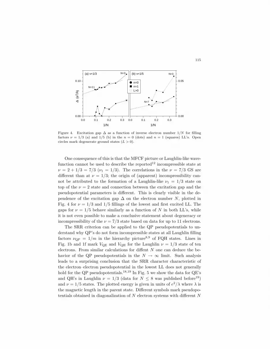
Figure 4. Excitation gap ∆ as a function of inverse electron number 1/N for fillingfactors ν = 1/3 (a) and 1/5 (b) in the n = 0 (dots) and n = 1 (squares) LL’s. Opencircles mark degenerate ground states (L > 0).

One consequence of this is that the MFCF picture or Laughlin-like wave-

function cannot be used to describe the reported12 incompressible state at

ν = 2 + 1/3 = 7/3 (ν1 = 1/3). The correlations in the ν = 7/3 GS are

different than at ν = 1/3; the origin of (apparent) incompressibility can-

not be attributed to the formation of a Laughlin-like ν1 = 1/3 state on

top of the ν = 2 state and connection between the excitation gap and the

pseudopotential parameters is different. This is clearly visible in the de-

pendence of the excitation gap ∆ on the electron number N , plotted in

Fig. 4 for ν = 1/3 and 1/5 fillings of the lowest and first excited LL. The

gaps for ν = 1/5 behave similarly as a function of N in both LL’s, while

it is not even possible to make a conclusive statement about degeneracy or

incompressibility of the ν = 7/3 state based on data for up to 11 electrons.

The SRR criterion can be applied to the QP pseudopotentials to un-

derstand why QP’s do not form incompressible states at all Laughlin filling

factors νQP = 1/m in the hierarchy picture8,9 of FQH states. Lines in

Fig. 1b and 1f mark VQE and VQH for the Laughlin ν = 1/3 state of ten

electrons. From similar calculations for diffent N one can deduce the be-

havior of the QP pseudopotentials in the N → ∞ limit. Such analysis

leads to a surprising conclusion that the SRR character characteristic of

the electron–electron pseudopotential in the lowest LL does not generally

hold for the QP pseudopotentials.18,19 In Fig. 5 we show the data for QE’s

and QH’s in Laughlin ν = 1/3 (data for N ≤ 8 was published before19)

and ν = 1/5 states. The plotted energy is given in units of e2/λ where λ is

the magnetic length in the parent state. Different symbols mark pseudopo-

tentials obtained in diagonalization of N electron systems with different N

116

0.10

0.15

E

(e2 /λ )

0.00

0.05(a) QE's in ν=1/3 (b) QH's in ν=1/3

1 3 5 7 9 11

0.01

0.04

E

(e2 /λ )

1 3 5 7 9 11

0.00

0.02

(c) QE's in ν=1/5 (d) QH's in ν=1/5

N=11 N=10N= 9N= 7 N= 6

N= 8

Figure 5. Energies of a pair of quasielectrons (left) and quasiholes (right) in Laughlinν = 1/3 (top) and ν = 1/5 (bottom) states, as a function of relative pair angularmomentum R, obtained in diagonalization of N electrons.

and thus with different lQP). Clearly, the QE and QH pseudopotentials are

quite different and neither one decreases monotonically with increasing R.

On the other hand, the corresponding pseudopotentials in ν = 1/3 and 1/5

states look similar, only the energy scale is different. The convergence of en-

ergies at small R obtained for larger N suggests that the maxima at R = 3

for QE’s and at R = 1 and 5 for QH’s, as well as the minima at R = 1 and

5 for QE’s and at R = 3 and 7 for QH’s, persist in the limit of large N (i.e.

for an infinite system on a plane). Consequently, the only incompressible

daughter states of Laughlin ν = 1/3 and 1/5 states are those with νQE = 1

or νQH = 1/3 (asterisks in Fig. 1) and (maybe) νQE = 1/5 and νQH = 1/7

(question marks in Fig. 1). It is also clear that no incompressible daughter

states will form at e.g. ν = 4/11 or 4/13. Taking into account the be-

havior of involved QP pseudopotentials on all levels of hierarchy explains

all observed odd-denominator FQH states and allows prediction of their

relative stability (without using trial wavefunctions involving multiple LL’s

and projections onto the lowest LL needed in Jain’s CF picture).

8. Conclusion

Using the pseudopotential formalism, we have described the FQH states in

terms of the ability of electrons to avoid strongly repulsive pair states. We

117

have defined the class of SRR pseudopotentials leading to the formation of

incompressible FQH states. We argue that the MFCF picture is justified

for the SRR interactions and fails for others. The pseudopotentials of the

Coulomb interaction in excited LL’s and of Laughlin QP’s in the ν = 1/3

state are shown to belong to the SRR class only at certain filling factors.

Acknowledgment

AW and JJQ acknowledge partial support by the Materials Research Pro-

gram of Basic Energy Sciences, US Department of Energy.

References

1. K. von Klitzing, G. Dorda, and M. Pepper, Phys. Rev. Lett. 45, 494 (1980).2. D. C. Tsui, H. L. Stormer, A. C. Gossard, Phys. Rev. Lett. 48, 1559 (1982).3. R. Laughlin, Phys. Rev. Lett. 50, 1395 (1983).4. The Quantum Hall Effect, edited by R. E. Prange and S. M. Girvin, Springer-

Verlag, New York (1987).5. F. D. M. Haldane and E. H. Rezayi, Phys. Rev. Lett. 60, 956 (1988).6. A. Wojs and J. J. Quinn, Solid State Commun. 108, 493 (1998); ibid. 110,

45 (1999); Philos. Mag. B80, 1405 (2000); J. J. Quinn, A. Wojs, J. Phys.:

Cond. Mat. 12, R265 (2000); A. Wojs, Phys. Rev. B63, 125312 (2001).7. A. de Shalit and I. Talmi, Nuclear Shell Theory, Academic Press, New York

(1963); R. D. Cowan, The Theory of Atomic Structure and Spectra, Univer-sity of California Press, Berkeley (1981).

8. F. D. M. Haldane, Phys. Rev. Lett. 51, 605 (1983).9. P. Sitko, K.-S. Yi, and J. J. Quinn, Phys. Rev. B 56, 12417 (1997).

10. S. Gasiorowicz, Quantum Physics, John Wiley and Sons, New York (1974).11. R. B. Laughlin, Surf. Sci. 142, 163 (1984); B. I. Halperin, Phys. Rev. Lett.

52, 1583 (1984); J. K. Jain and V. J. Goldman, Phys. Rev. B45, 1255 (1992).12. R. Willet, J. P. Eisenstein, H. L. Stormer, D. C. Tsui, A. C. Gossard, and J.

H. English, Phys. Rev. Lett. 59, 1776 (1987).13. J. R. Mallet, R. G. Clark, R. J. Nicholas, R. L. Willet, J. J. Harris, and C.

T. Foxon, Phys. Rev. B38, 2200 (1988); T. Sajoto, Y. W. Suen, L. W. Engel,M. B. Santos, and M. Shayegan, Phys. Rev. B41, 8449 (1990).

14. J. Jain, Phys. Rev. Lett. 63, 199 (1989).15. A. Lopez and E. Fradkin, Phys. Rev. B44, 5246 (1991).16. T. T. Wu and C. N. Yang, Nucl. Phys. B107, 365 (1976).17. X. M. Chen and J. J. Quinn, Solid State Commun. 92, 865 (1996).18. P. Beran and R. Morf, Phys. Rev. B43, 12654 (1991).19. S. N. Yi, X. M. Chen, and J. J. Quinn, Phys. Rev. B53, 9599 (1996).