Identification of source of a marine oil-spill using geochemical and chemometric techniques Marcio M. Lobão a , Jari N. Cardoso b,⇑ , Marcio R. Mello c , Paul W. Brooks c , Claudio C. Lopes b , Rosangela S.C. Lopes b a Institute of Sea Studies Adm. Paulo Moreira (IEAPM), Arraial do Cabo, Brazil b Institute of Chemistry, Federal University of Rio de Janeiro, Cidade Universitaria, Ilha do Fundão, Bloco A, P.O. 21949-900, Rio de Janeiro, Brazil c HRT Petroleum Ltd., Av. Atlantica, 1130, 7th floor, P.O. 22060-000, Rio de Janeiro, Brazil article info Keywords: Oil-spill Brazil San Marcos bay d 13 C Ni/V Biomarker abstract The current work aimed to identify the source of an oil spill off the coast of Maranhão, Brazil, in Septem- ber 2005 and effect a preliminary geochemical survey of this environment. A combination of bulk analyt- ical parameters, such as carbon isotope (d 13 C) and Ni/V ratios, and conventional fingerprinting methods (High Resolution Gas Chromatography and Mass Spectrometry) were used. The use of bulk methods greatly speeded source identification for this relatively unaltered spill: identification of the likely source was possible at this stage. Subsequent fingerprinting of biomarker distributions supported source assign- ment, pointing to a non-Brazilian oil. Steranes proved the most useful biomarkers for sample correlation in this work. Distribution patterns of environmentally more resilient compound types, such as certain aromatic structures, proved inconclusive for correlation, probably in view of their presence in the background. Ó 2010 Elsevier Ltd. All rights reserved. 1. Introduction Petroleum can seep into the surface by natural causes and re- ports of surficial oil occurrences date back to ancient civilizations (Boëda et al., 1996). Such occurrences have never been the cause of more than historical interest, restricted as they have been in number, volume of the spill and local impact of the seep. It was only after petroleum became the world’s main source of energy, following massive industrialization in contemporary societies, that exploitation, transport and storage of this resource became proba- bly the main source of exogenous organic compounds into the environment (Wang et al., 1999; Meniconi et al., 2002; Wang and Fingas, 2003). Transport of the crude or sub-fractions over international or intercontinental distances, in particular, has be- come a major source of environmental risk and concern. Dramatic in their impact, massive spills pose no problems as regards identi- fication of source and responsibilities. It is now possible, with modern satellite imagery, for example, to spot the spill and its propagation in real time, making containment measures and assignment of responsibilities reasonably easy (e.g., Shaban et al., 2009). It is usually the (relatively) small-scale, chronic contamina- tion introduced, almost daily, by ships discharging ballast water, washing oil tanks and, especially, by accidents during the opera- tions of loading/unloading tankers and by leakage from pipelines that, in view of the variety of possible sources, can pose a challenge to the correlation work of the forensic analyst (Stout et al., 2001). The problem can be further aggravated by changes in composition of the oil once released into the environment (Barakat et al., 2002). Identification of the source of spills relies usually on comparison of the molecular composition of the oil with that of suspected sources, similarly to the traditional routines used in geochemistry for correlating different oils or oils to source-rocks (Mello et al., 1990; Stout et al., 2001; Daling et al., 2002; Peters et al., 2005; Wang et al., 2006), with extensive use of GC and GC–MS for mon- itoring occurrence and distribution of characteristic families of compounds (biomarkers) in the samples to be compared. The current work was the result of such a study: an off-shore oil spill occurred in the bay of San Marcos (state of Maranhão, northern Brazil) in September 2005 with impact on local beaches (all located in San Louis island, Fig. 1). Major commercial ship terminals, mostly for export, such as Itaqui (liquid bulk, pig iron, aluminium), Alumar (bauxite), Madeira Point and CVRD (iron ore) are located inside the bay, benefitting from the deep water access channel (ca. 27 m), which favours intense traffic of large ships, including oil tankers. The bay itself is part of a macrotidal gulf zone, with spring tides ranging from 0.3 to 7.1 m and currents that can reach 5–6 knots, 2–3 h after commencement of flood tide (Alcantara and Santos, 2005), carrying suspended sediment and contaminants out 0025-326X/$ - see front matter Ó 2010 Elsevier Ltd. All rights reserved. doi:10.1016/j.marpolbul.2010.08.008 ⇑ Corresponding author. Tel.: +55 25627553; fax: +55 2562 7262. E-mail address: [email protected](J.N. Cardoso). Marine Pollution Bulletin 60 (2010) 2263–2274 Contents lists available at ScienceDirect Marine Pollution Bulletin journal homepage: www.elsevier.com/locate/marpolbul
Identification of source of a marine oil-spill using geochemical andchemometric techniques
Marcio M. Lobão a, Jari N. Cardoso b,⇑, Marcio R. Mello c, Paul W. Brooks c, Claudio C. Lopes b,Rosangela S.C. Lopes b
a Institute of Sea Studies Adm. Paulo Moreira (IEAPM), Arraial do Cabo, Brazilb Institute of Chemistry, Federal University of Rio de Janeiro, Cidade Universitaria, Ilha do Fundão, Bloco A, P.O. 21949-900, Rio de Janeiro, Brazilc HRT Petroleum Ltd., Av. Atlantica, 1130, 7th floor, P.O. 22060-000, Rio de Janeiro, Brazil
The current work aimed to identify the source of an oil spill off the coast of Maranhão, Brazil, in Septem-ber 2005 and effect a preliminary geochemical survey of this environment. A combination of bulk analyt-ical parameters, such as carbon isotope (d13C) and Ni/V ratios, and conventional fingerprinting methods(High Resolution Gas Chromatography and Mass Spectrometry) were used. The use of bulk methodsgreatly speeded source identification for this relatively unaltered spill: identification of the likely sourcewas possible at this stage. Subsequent fingerprinting of biomarker distributions supported source assign-ment, pointing to a non-Brazilian oil. Steranes proved the most useful biomarkers for sample correlationin this work. Distribution patterns of environmentally more resilient compound types, such as certainaromatic structures, proved inconclusive for correlation, probably in view of their presence in thebackground.
� 2010 Elsevier Ltd. All rights reserved.
1. Introduction
Petroleum can seep into the surface by natural causes and re-ports of surficial oil occurrences date back to ancient civilizations(Boëda et al., 1996). Such occurrences have never been the causeof more than historical interest, restricted as they have been innumber, volume of the spill and local impact of the seep. It wasonly after petroleum became the world’s main source of energy,following massive industrialization in contemporary societies, thatexploitation, transport and storage of this resource became proba-bly the main source of exogenous organic compounds into theenvironment (Wang et al., 1999; Meniconi et al., 2002; Wangand Fingas, 2003). Transport of the crude or sub-fractions overinternational or intercontinental distances, in particular, has be-come a major source of environmental risk and concern. Dramaticin their impact, massive spills pose no problems as regards identi-fication of source and responsibilities. It is now possible, withmodern satellite imagery, for example, to spot the spill and itspropagation in real time, making containment measures andassignment of responsibilities reasonably easy (e.g., Shaban et al.,2009). It is usually the (relatively) small-scale, chronic contamina-tion introduced, almost daily, by ships discharging ballast water,
ll rights reserved.
55 2562 7262.
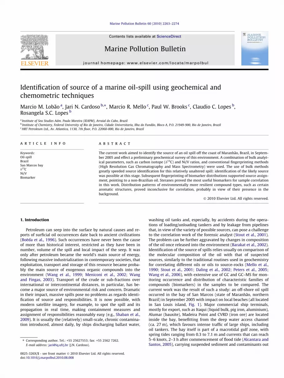
washing oil tanks and, especially, by accidents during the opera-tions of loading/unloading tankers and by leakage from pipelinesthat, in view of the variety of possible sources, can pose a challengeto the correlation work of the forensic analyst (Stout et al., 2001).The problem can be further aggravated by changes in compositionof the oil once released into the environment (Barakat et al., 2002).Identification of the source of spills relies usually on comparison ofthe molecular composition of the oil with that of suspectedsources, similarly to the traditional routines used in geochemistryfor correlating different oils or oils to source-rocks (Mello et al.,1990; Stout et al., 2001; Daling et al., 2002; Peters et al., 2005;Wang et al., 2006), with extensive use of GC and GC–MS for mon-itoring occurrence and distribution of characteristic families ofcompounds (biomarkers) in the samples to be compared. Thecurrent work was the result of such a study: an off-shore oil spilloccurred in the bay of San Marcos (state of Maranhão, northernBrazil) in September 2005 with impact on local beaches (all locatedin San Louis island, Fig. 1). Major commercial ship terminals,mostly for export, such as Itaqui (liquid bulk, pig iron, aluminium),Alumar (bauxite), Madeira Point and CVRD (iron ore) are locatedinside the bay, benefitting from the deep water access channel(ca. 27 m), which favours intense traffic of large ships, includingoil tankers. The bay itself is part of a macrotidal gulf zone, withspring tides ranging from 0.3 to 7.1 m and currents that can reach5–6 knots, 2–3 h after commencement of flood tide (Alcantara andSantos, 2005), carrying suspended sediment and contaminants out
to sea. This scenario probably explains why the major impact of the2005 spill, occurred outside the bay, on adjacent oceanic beaches,such as São Marcos, Calhau and Do Meio, otherwise pristine coastalareas (see Fig. 1).
2. Materials and methods
2.1. Sampling
Samples were collected manually in September 2005 onboardvarious suspect ships (anchored or navigating at São Marcos Bayduring the spill, see list on Table 1) by taking 50–100 mg of theoil into glass flasks and diluting with 1 ml of n-hexane. Storagewas at room temperature until analysis. This was the case of shipsamples (AET01–AET014). Samples AET015, AET016 and AET017were from the actual spilled oil + sand collected on the beaches:ca. 30 g of sand impregnated with oil were mixed with 20 g ofanhydrous sodium sulphate (to remove water), ultrasonically ex-tracted (dichloromethane, 3 � 50 ml) and centrifuged. Extractswere concentrated to 5 ml on a rotary evaporator (Wang et al.,1994).
2.2. Sample preparation
Excepting the beach samples, very little treatment was done onthe collected samples to avoid fractionation and a change in their
original composition. HRGC analyses (whole oil) involved dilutionof ca. 50–100 mg of the sample in 1 ml of n-hexane. HRGC–MS in-volved fractionation of the sample (50–100 mg) by gravity liquidchromatography on glass columns (1.2 � 30 cm) packed with20 g of silica-gel topped with 1 g of sodium sulphate. The saturate
fraction was obtained by percolation with 40 ml of n-hexane andthe aromatics by subsequent elution with 40 ml of a solution ofn-hexane/dichloromethane (3/1, v/v). Both fractions were takento dryness in a rotary evaporator and redissolved in 200 ll of sol-vent prior to analysis.
2.3. Solvents and reagents
For extraction, drying and fractionation of the oils, the followingsolvents and reagents were used as received, without furtherpurification:
- Oil AEN 0026, made available by HRT & Petroleum Technologies(RJ), was used as standard for HRGC–FID whole oil analyses.This is an undegraded sample of oil used for optimizing GCconditions and calibrating retention times of individualbiomarkers.
- Identification by HRGC–MS of the various individual biomark-ers present in the suspected sources and spill was done by com-parison of retention times in the appropriate massfragmentograms with data from previous analyses of referenceoils (HRT & Petroleum Technologies, RJ) run under the sameconditions. Quantitation was performed by automated peakheight measurement.
- C12/C13 analyses of the samples were carried out by isotoperatio mass spectrometry and used oil 1-RJS-359 as a surrogatestandard (d13C = �24.20% versus PDB).
- Analyses of nickel and vanadium used, as references, solutionsof the multi-element standard Conostan S-21 (Conoco Inc.,USA).
2.5. High resolution gas chromatography (HRGC)
An Agilent 6890 (USA) gas chromatograph fitted with a fused-silica capillary column (0.25 mm � 30 m) coated with a film(0.25 lm) of DB-1 (100% methyl-silicone), was used, followingNorm EPA 8051B. Samples were injected without any prior frac-tionation (whole oil). Detection was by FID, using helium as carrier(16 psi inlet pressure) and sample injection (1 ll) was in the split-less mode. Initial temperature was 50 �C, with gradient of 6�/minup to a final temperature of 310 �C (10 min hold). Detector temper-ature was 280 �C. Peak assignments were by retention time andabundances by peak height measurement compared to a referenceoil sample, as mentioned previously. Pristane/phytane, pristane/n-C17, phytane/n-C18, n-C20/n-C25, n-C28/n-C30 and n-C25/n-C30 ratios were calculated automatically by the instrumentworkstation.
2.6. Nickel/vanadium ratios
Determination of the levels of nickel and vanadium was as de-scribed by Brown (1983), in conformity with Norm ASTM D5708a,1995. All samples were dissolved in xylene (1/10, v/v) and ana-lyzed in triplicate on a Perkin-Elmer Plasma 1000 ICP-OES (USA),using Conostan S-21 as reference standard, under the followingconditions: wavelengths Ni(I) 231.604 nm and V(II) 292.402 nm.Detection limits were 0.010 and 0.002 mg/kg, respectively. Argon
and sample flows into the plasma were 15 and 1.0 l/min, respec-tively, with an rf value of 27.12 MHz.
2.7. Determination of carbon isotope ratios
d13C analyses were done without any separation of individualcomponents (whole oil). Isotope ratios were measured on a Finni-gan MAT 252 mass spectrometer (USA) after combustion for con-version of samples to CO2. All samples were analyzed intriplicate and the results averaged.
2.8. HRGC–MS analyses
Characterization of individual components in saturate and aro-matic fractions was performed on an Agilent 6890 gas chromato-graph coupled to a 5973 mass spectrometer. Chromatographiccolumn was a fused-silica capillary (60 m � 0.25 mm) coated witha 0.25 lm film of DB-5 (5% phenyl–95% methyl polysyloxane). Onlythe actual spilled oil (AET015) was analyzed in triplicate (generat-ing samples AET016 and AET017) to check for analytical variations,as recommended (Stout et al., 2001; Daling et al., 2002). Chromato-graphic conditions for analyses of alkanes were: 55 �C as initialtemperature (2 min hold) followed by a 20 �C/min increase up to150 �C, with a second gradient (1,5 �C/min) up to 320 �C (5 minhold). Ion source and quadrupole temperatures were 230 and150 �C, respectively. Sample size was 2 lL injected under splitlessconditions. Data acquisition was in the SIM mode. The GC oventemperature programme for analysis of aromatics was: 50 �C asinitial temperature (2 min hold), 6 �C/min gradient up to 310 �C(15 min hold-up time). Sample size was 2 lL, mode of injectionwas splitless, quadrupole and detector temperatures were 230and 150 �C, respectively. The list of ions to be monitored by massspectrometry was as usually reported on correlation studies ofoil-spills (Douglas et al., 1996; Barakat et al., 1999; Wang et al.,1999, 2006; Barakat et al., 2001, 2002; Daling et al. 2002; Stoutet al., 2001; Peters et al., 2005) and covered straight-chain/branched alkanes and ubiquitous petroleum polycyclic structuressuch as tricyclic and pentacyclic terpanes, steranes (regular, meth-ylated, degraded and rearranged) as well as polynuclear aromatichydrocarbons (parent compounds and alkylated homologs). Thedistribution of such structures was obtained by screening the elu-tion profiles of characteristic fragment ions (mass fragmento-grams). Rather than use quantitative values for individualcomponents, ratios between values (diagnostic ratios – Rd) havebeen found more useful for correlation and were adopted, in keep-ing with general practice.
2.9. Multivariate treatment of data
Principal Component Analysis (PCA) (Burns et al., 1997; Stoutet al., 2001; Stella et al., 2002; Peters et al., 2005; Christensenet al., 2005) and Hierarchical Cluster Analysis (HCA) (Meniconiet al., 2002; Hosttetler et al., 2004) were used for correlation ofthe various Rd. Pre-treatment (normalization) of the raw data(parameter ratios – Rd) to a common variance value, as recom-mended (Massart et al., 1997; Miller and Miller, 2000) was used,to avoid false enhancement of certain parameters, presenting largedifferences in variances, in the subsequent multivariate data anal-ysis. It became evident, during application, that ranking of Rd’sbased on their capacity to discriminate samples, as proposed inthe literature (Christensen et al., 2004), was very useful in afford-ing plots showing a clearer relationship between clusters andadopted in this work. Obviously, in view of the extensive amountof data, multivariate analyses could only be efficiently performedwith the aid of computer software: MVSP (a multi-variate statisti-cal package for HCA and dispersion plots) was available, for
evaluation purposes, on site www.kovcomp.co.uk (access in02/01/2007).
3. Results and discussion
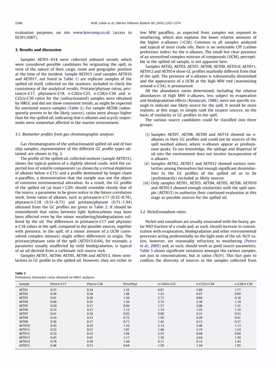
Samples AET01–014 were collected onboard vessels whichwere considered possible candidates for originating the spill, inview of the nature of their cargo, route and geographic positionat the time of the incident. Sample AET015 (and samples AET016and AET017, not listed in Table 1) are replicate samples of thespilled oil itself, collected on the seashore, included to check theconsistency of the analytical results. Pristane/phytane ratios, pris-tane/n-C17, phytane/n-C18, n-C20/n-C25, n-C28/n-C30 and n-C25/n-C30 ratios for the (unfractionated) samples were obtainedby HRGC and did not show consistent trends, as might be expectedfor unrelated source samples (Table 2). For sample AET06 (subse-quently proven to be the likely source), ratios were always higherthan for the spilled oil, indicating that n-alkanes and acyclic isopre-noids were somewhat affected in the marine environment.
3.1. Biomarker profiles from gas chromatographic analyses
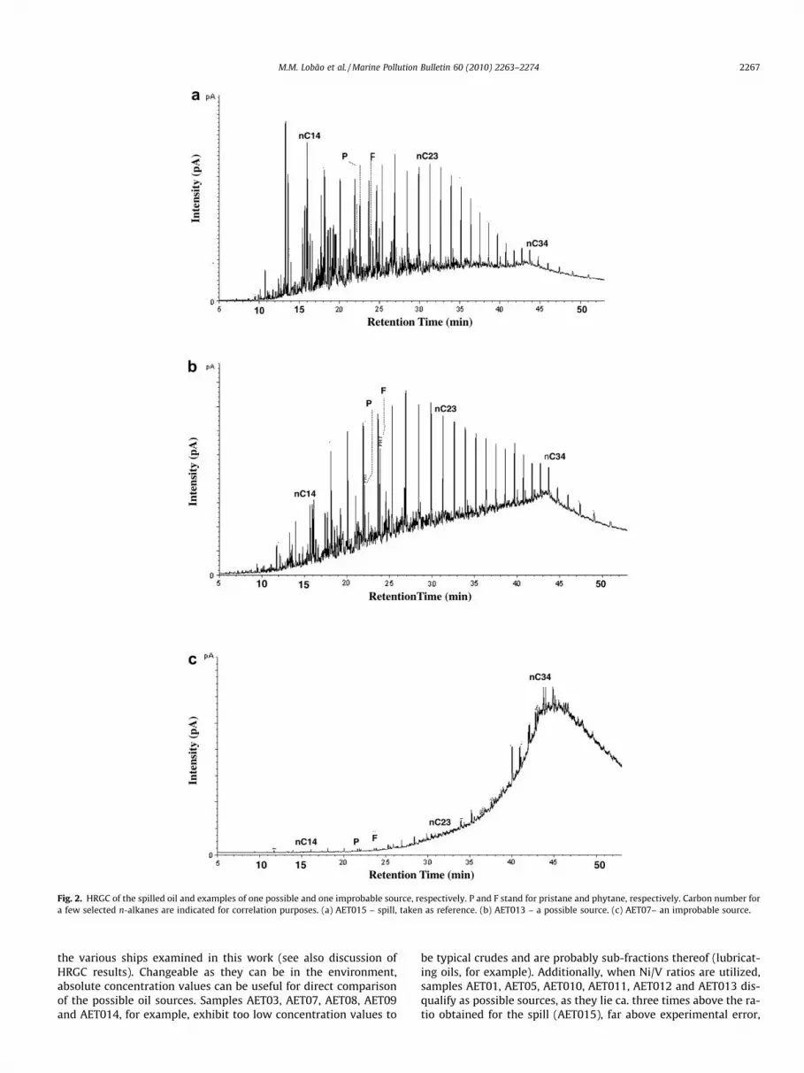
Gas chromatograms of the unfractionated spilled oil and of twoship samples, representative of the different GC profile types ob-tained, are shown in Fig. 2.
The profile of the spilled oil, collected onshore (sample AET015),shows the typical pattern of a slightly altered crude, with the ex-pected loss of volatile components (as shown by a virtual depletionof alkanes below n-C15) and a profile dominated by longer-chainn-paraffins, a demonstration that the sample was not the objectof extensive environmental alteration. As a result, the GC profileof the spilled oil (at least > C20) should resemble closely that ofthe source, a parameter to be given notice in the future correlationwork. Some ratios of alkanes, such as pristane/n-C17 (0.32–0.78),phytane/n-C18 (0.31–0.73) and pristane/phytane (0.71–1.94)obtained from the GC profiles are given in Table 2. It should beremembered that ratios between light hydrocarbons may havebeen affected even by the minor weathering/biodegradation suf-fered by the oil. The differences in pristane/n-C17 and phytane/n-C18 values in the spill, compared to the possible sources, togetherwith presence, in the spill, of a minor amount of a UCM (unre-solved complex mixture) might reflect differences in origin. Thepristane/phytane ratio of the spill (AET015:0.64), for example, aparameter usually unaffected by mild biodegradation, is typicalof an oil derived from a carbonate rich source rock.
Samples AET01, AET04, AET05, AET06 and AET013, show simi-larities in GC profile to the spilled oil. However, they are richer in
Table 2Preliminary biomarker ratios obtained on HRGC analyses.
low MW paraffins, as expected from samples not exposed toweathering, which also explains the lower relative amounts ofthe higher n-alkanes (>C20). Common to all samples analyzedand typical of most crude oils, there is no noticeable CPI (carbonpreference index) for the n-alkanes. The small but clear presenceof an unresolved complex mixture of compounds (UCM), percepti-ble in the spilled oil sample, is not apparent here.
Samples AET02, AET03, AET07, AET08, AET09, AET010, AET011,AET012 and AET014 show GC profiles markedly different from thatof the spill. The presence of n-alkanes is substantially diminishedand the appearance of a UCM at the high MW end (maximizingaround n-C34), is pronounced.
All the abundance ratios determined, including the relativeabundances of high MW n-alkanes, less subject to evaporationand biodegradation effects (Kennicutt, 1988), were not specific en-ough to indicate one likely source for the spill. It would be morerealistic, at this stage, to simply rank the suspect sources, on thebasis of similarity in GC profiles to the spill.
The various source candidates could be classified into threegroups:
(i) Samples AET07, AET08, AET09 and AET14 showed no n-alkanes in their GC profiles and could not be sources of thespill washed ashore, where n-alkanes appear as predomi-nant peaks. To our knowledge, the spillage and dispersal ofoil into the environment does not involve incorporation ofn-alkanes.
(ii) Samples AET02, AET011 and AET012 showed various simi-larities among themselves but enough significant dissimilar-ities to the GC profiles of the spilled oil as to be(preliminarily) excluded as likely sources.
(iii) Only samples AET01, AET03, AET04, AET05, AET06, AET010and AET013 showed enough similarities with the spill sam-ple (AET015) to authorize their continued evaluation at thisstage as possible sources for the spilled oil.
3.2. Nickel/vanadium ratios
Nickel and vanadium are usually associated with the heavy, po-lar NSO fraction of a crude and, as such, should increase in concen-tration with evaporation, biodegradation and other environmentalprocesses acting preferentially on the light ends of the oil. Ni/V ra-tios, however, are reasonably refractory to weathering (Peterset al., 2005) and, as such, should work as good source parameters.Table 3 shows significant variations amongst the various samples,not just in concentrations, but in ratios (Ni/V). This fact goes toconfirm the diversity of sources in the samples collected from
Fig. 2. HRGC of the spilled oil and examples of one possible and one improbable source, respectively. P and F stand for pristane and phytane, respectively. Carbon number fora few selected n-alkanes are indicated for correlation purposes. (a) AET015 – spill, taken as reference. (b) AET013 – a possible source. (c) AET07– an improbable source.
the various ships examined in this work (see also discussion ofHRGC results). Changeable as they can be in the environment,absolute concentration values can be useful for direct comparisonof the possible oil sources. Samples AET03, AET07, AET08, AET09and AET014, for example, exhibit too low concentration values to
be typical crudes and are probably sub-fractions thereof (lubricat-ing oils, for example). Additionally, when Ni/V ratios are utilized,samples AET01, AET05, AET010, AET011, AET012 and AET013 dis-qualify as possible sources, as they lie ca. three times above the ra-tio obtained for the spill (AET015), far above experimental error,
Table 3Nickel and vanadium content in spill and possible sources.
and the statistical analytical confidence limits (e.g., 95%). SamplesAET02 (no match by HRGC), AET04 and AET06 remain as the onlysamples which could possibly have sourced the spill. As Ni/V anal-yses are rapid, requiring no sample preparation, this discussionshows that they can be very useful in screening large numbers ofsamples.
3.3. Carbon isotope (d13C) isotope analyses
Carbon isotope ratios reported in this work were determined forthe whole (unfractionated) samples, and the results reported(Table 4) should be regarded as average values, taking into accountthat differences in isotope ratios have been reported amongst thevarious fractions in geological samples (Murray et al., 1994). Evenso, the use of bulk isotope ratios has proved useful in correlations,as the action of physical environmental parameters in a spill, suchas weathering, water-washing and evaporation, does not have asignificant effect in carbon isotope signatures, whereas biodegra-dation, especially where major loss of certain isotopic – light struc-tures, such as n-alkanes is involved, usually does (Jeffrey, 2006). Asheavy biodegradation is not involved in the present case, the vari-ations shown are most likely the result of different sources for theoils, when compared to the spill. Adopting the 95% confidence limitproposed by Peters et al. (2005), only samples AET03, AET04,AET06, AET07, AET08, AET09 and AET10 would be related to thespill (AET015). As samples AET07, AET08 and AET09 were dis-carded on the basis of GC profiles (see previously), only AET03,
Table 4Carbon isotope ratios (d13C‰) in spill and possiblesources.a
a All values were obtained on unfractionated samples(whole oils).
AET04, AET06 and AET010 would remain as possibilities. If the re-sults of Ni/V ratios are also incorporated, AET04 and AET06 becomethe most likely sources.
3.4. HRGC–MS analyses
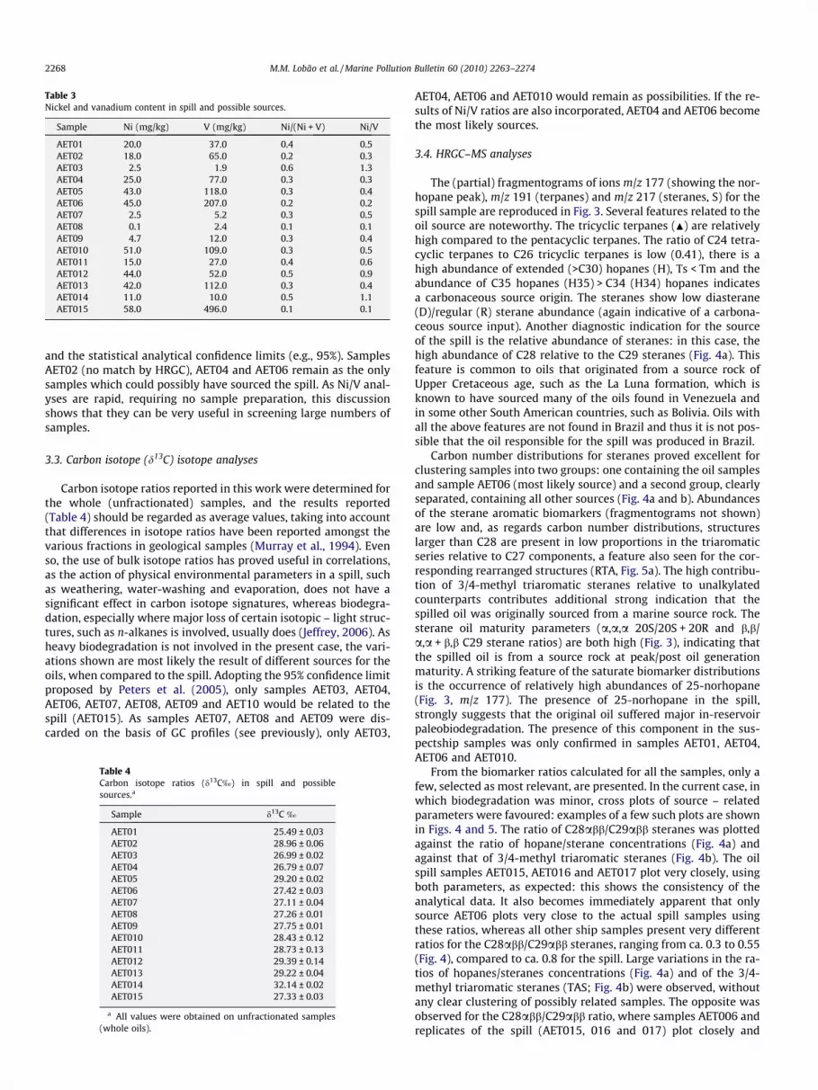
The (partial) fragmentograms of ions m/z 177 (showing the nor-hopane peak), m/z 191 (terpanes) and m/z 217 (steranes, S) for thespill sample are reproduced in Fig. 3. Several features related to theoil source are noteworthy. The tricyclic terpanes (N) are relativelyhigh compared to the pentacyclic terpanes. The ratio of C24 tetra-cyclic terpanes to C26 tricyclic terpanes is low (0.41), there is ahigh abundance of extended (>C30) hopanes (H), Ts < Tm and theabundance of C35 hopanes (H35) > C34 (H34) hopanes indicatesa carbonaceous source origin. The steranes show low diasterane(D)/regular (R) sterane abundance (again indicative of a carbona-ceous source input). Another diagnostic indication for the sourceof the spill is the relative abundance of steranes: in this case, thehigh abundance of C28 relative to the C29 steranes (Fig. 4a). Thisfeature is common to oils that originated from a source rock ofUpper Cretaceous age, such as the La Luna formation, which isknown to have sourced many of the oils found in Venezuela andin some other South American countries, such as Bolivia. Oils withall the above features are not found in Brazil and thus it is not pos-sible that the oil responsible for the spill was produced in Brazil.
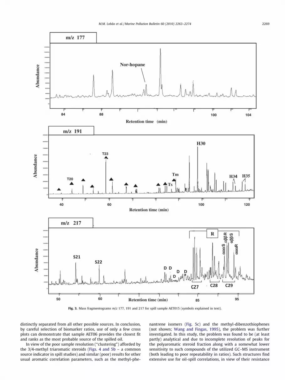
Carbon number distributions for steranes proved excellent forclustering samples into two groups: one containing the oil samplesand sample AET06 (most likely source) and a second group, clearlyseparated, containing all other sources (Fig. 4a and b). Abundancesof the sterane aromatic biomarkers (fragmentograms not shown)are low and, as regards carbon number distributions, structureslarger than C28 are present in low proportions in the triaromaticseries relative to C27 components, a feature also seen for the cor-responding rearranged structures (RTA, Fig. 5a). The high contribu-tion of 3/4-methyl triaromatic steranes relative to unalkylatedcounterparts contributes additional strong indication that thespilled oil was originally sourced from a marine source rock. Thesterane oil maturity parameters (a,a,a 20S/20S + 20R and b,b/a,a + b,b C29 sterane ratios) are both high (Fig. 3), indicating thatthe spilled oil is from a source rock at peak/post oil generationmaturity. A striking feature of the saturate biomarker distributionsis the occurrence of relatively high abundances of 25-norhopane(Fig. 3, m/z 177). The presence of 25-norhopane in the spill,strongly suggests that the original oil suffered major in-reservoirpaleobiodegradation. The presence of this component in the sus-pectship samples was only confirmed in samples AET01, AET04,AET06 and AET010.
From the biomarker ratios calculated for all the samples, only afew, selected as most relevant, are presented. In the current case, inwhich biodegradation was minor, cross plots of source – relatedparameters were favoured: examples of a few such plots are shownin Figs. 4 and 5. The ratio of C28abb/C29abb steranes was plottedagainst the ratio of hopane/sterane concentrations (Fig. 4a) andagainst that of 3/4-methyl triaromatic steranes (Fig. 4b). The oilspill samples AET015, AET016 and AET017 plot very closely, usingboth parameters, as expected: this shows the consistency of theanalytical data. It also becomes immediately apparent that onlysource AET06 plots very close to the actual spill samples usingthese ratios, whereas all other ship samples present very differentratios for the C28abb/C29abb steranes, ranging from ca. 0.3 to 0.55(Fig. 4), compared to ca. 0.8 for the spill. Large variations in the ra-tios of hopanes/steranes concentrations (Fig. 4a) and of the 3/4-methyl triaromatic steranes (TAS; Fig. 4b) were observed, withoutany clear clustering of possibly related samples. The opposite wasobserved for the C28abb/C29abb ratio, where samples AET006 andreplicates of the spill (AET015, 016 and 017) plot closely and
m/z 191
Nor-hopane
H34 H35
m/z 217
R
Retention time (min)
Retention time (min)
Retention time (min)
Abu
ndan
ce
Ts
Tm
H30
60 50 85 95
84 88 100 104
40 60 100 120
T23
T20
D
RSR S
Abu
ndan
ceA
bund
ance
Fig. 3. Mass fragmentograms m/z 177, 191 and 217 for spill sample AET015 (symbols explained in text).
distinctly separated from all other possible sources. In conclusion,by careful selection of biomarker ratios, use of only a few crossplots can demonstrate that sample AET06 provides the closest fitand ranks as the most probable source of the spilled oil.
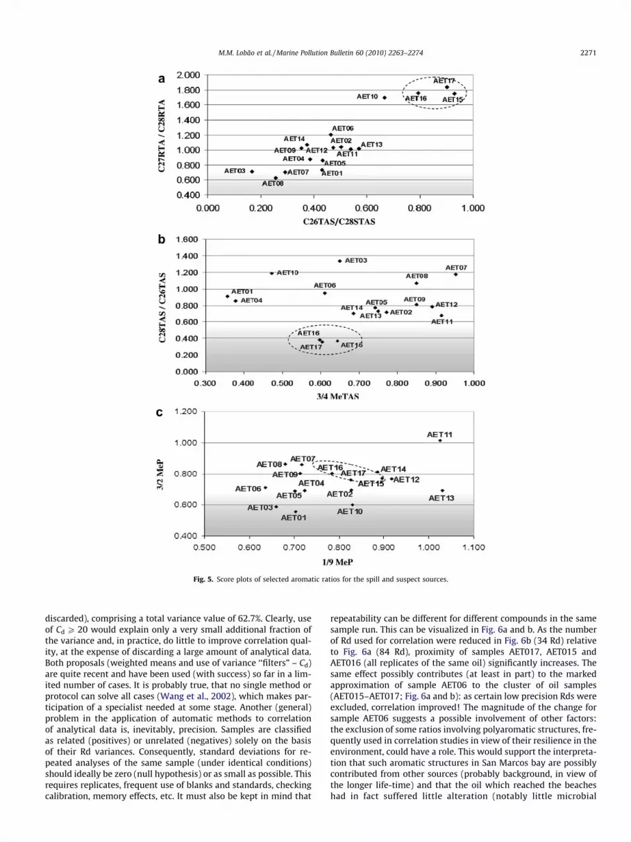
In view of the poor sample resolution (‘‘clustering”) afforded bythe 3/4-methyl triaromatic steroids (Figs. 4 and 5b – a commonsource indicator in spill studies) and similar (poor) results for otherusual aromatic correlation parameters, such as the methyl-phe-
nantrene isomers (Fig. 5c) and the methyl-dibenzothiophenes(not shown; Wang and Fingas, 1995), the problem was furtherinvestigated. In this study, the problem was found to be (at leastpartly) analytical and due to incomplete resolution of peaks forthe polyaromatic steroid fraction along with a somewhat lowersensitivity to such compounds of the utilized GC–MS instrument(both leading to poor repeatability in ratios). Such structures findextensive use for oil-spill correlations, in view of their resistance
AET0001
AET0002AET0003
AET0004AET0005
AET0006
AET0007AET0008
AET0009
AET0010
AET0011
AET0012AET0013
AET0014
AET0015
AET0016
AET0017
0.00
0.10
0.20
0.30
0.40
0.50
0.60
0.70
0.80
0.90
0.00 5.00 10.00 15.00 20.00 25.00
Hopanes/Steranes
C28
bb/
C29
bb s
tera
nes
3/4 MeTAS
C28
bb/C
29bb
ste
rane
s
a
b
Fig. 4. Score plots of hopane and sterane ratios for spill and suspect sources.
to weathering in the environment (e.g., Wang et al., 2006). The po-tential of MS–MS (not available in this work) to get around theanalytical problems, as recommended by Peters et al. (2005), couldnot be evaluated. The problem is further discussed under PCAanalyses.
3.5. Automatic multivariate analyses
The multivariate analyses performed in this study used PCA(principal component analyses) and HCA (hierarchical componentanalyses) methods, as usual in most types of geochemical correla-tion work. The following ions (m/z values), characteristic of thestructural classes analyzed, were used: 177.191 (triterpanes), 205(C1-triterpanes), 217.218 (steranes), 259 (diasteranes), 178.192(C0–C1-phenanthrenes), 184.198 (C0–C1-dibenzothiophenes),231.245 (C0–C1-triaromatic steroids). Extensive combination ofthe abundances of single components (or a range of homologues)within each homologous series, as well as ratios between differentstructural types (single components or sum of homologues) wasemployed to generate the range of diagnostic ratios, as usual (forfurther discussion, see, for example, Daling et al., 2002; Faksnesset al., 2002; Christensen et al., 2004; Peters et al., 2005; Wanget al., 2006). Eighty-four Rd’s were developed. Irrespective ofthe type of multivariate analysis employed, raw data were pre-processed (standardized) to zero mean and unit variance (Miller
and Miller, 2000) so that each variable carries equal weight inthe statistical treatment.
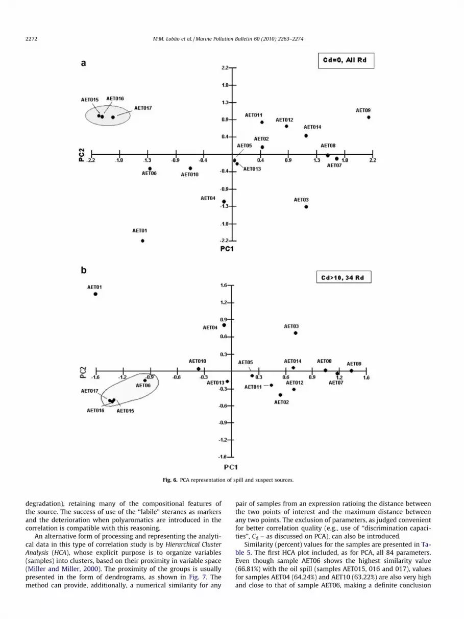
Initially, all 84 Rd (51.2% of the total variance) were used forcorrelation by Principal Component Analysis (PCA) of all samples(Fig. 6). The proximity of samples AET06 and AET10 to the clusterof samples of the oil (AET015, AET016 and AET017) becomesimmediately obvious, in one step, indicating the two samples asthe most likely sources for the spill, a conclusion reached only afterdetailed interpretation of GC–MS analyses, as discussed previously.Despite the speed and convenience, essential in the heavy work-load of an environmental lab, indiscriminate application of auto-matic methods can lead to errors. The problem of combiningparameters with large differences in variance has been handled,for example, by modifications in the computer algorithms, suchas the use of weighted mean squares (Bro et al., 2002), or the intro-duction of ‘‘discrimination capacity” (Cd), a factor defined as the ra-tio of relative standard deviations between possible sources andspill (Christensen et al., 2004). The latter method (used in thiswork) functions as a filter and implies in rejection of ratios withsmall variances, with a consequent decrease in the number of vari-ables used for correlation. Examples are shown in Fig. 6(b), whereonly Cd P 10 are represented: the set of samples is as in Fig. 6(a)but now 50 ratios (Rd) were discarded and the plots involved only34 Rd, comprising 61.6% of the total variance (PC1 + PC2). For a va-lue of Cd P 20 (plot not shown), only 21 Rd would be used (and 63
Fig. 5. Score plots of selected aromatic ratios for the spill and suspect sources.
discarded), comprising a total variance value of 62.7%. Clearly, useof Cd P 20 would explain only a very small additional fraction ofthe variance and, in practice, do little to improve correlation qual-ity, at the expense of discarding a large amount of analytical data.Both proposals (weighted means and use of variance ‘‘filters” – Cd)are quite recent and have been used (with success) so far in a lim-ited number of cases. It is probably true, that no single method orprotocol can solve all cases (Wang et al., 2002), which makes par-ticipation of a specialist needed at some stage. Another (general)problem in the application of automatic methods to correlationof analytical data is, inevitably, precision. Samples are classifiedas related (positives) or unrelated (negatives) solely on the basisof their Rd variances. Consequently, standard deviations for re-peated analyses of the same sample (under identical conditions)should ideally be zero (null hypothesis) or as small as possible. Thisrequires replicates, frequent use of blanks and standards, checkingcalibration, memory effects, etc. It must also be kept in mind that
repeatability can be different for different compounds in the samesample run. This can be visualized in Fig. 6a and b. As the numberof Rd used for correlation were reduced in Fig. 6b (34 Rd) relativeto Fig. 6a (84 Rd), proximity of samples AET017, AET015 andAET016 (all replicates of the same oil) significantly increases. Thesame effect possibly contributes (at least in part) to the markedapproximation of sample AET06 to the cluster of oil samples(AET015–AET017; Fig. 6a and b): as certain low precision Rds wereexcluded, correlation improved! The magnitude of the change forsample AET06 suggests a possible involvement of other factors:the exclusion of some ratios involving polyaromatic structures, fre-quently used in correlation studies in view of their resilience in theenvironment, could have a role. This would support the interpreta-tion that such aromatic structures in San Marcos bay are possiblycontributed from other sources (probably background, in view ofthe longer life-time) and that the oil which reached the beacheshad in fact suffered little alteration (notably little microbial
Fig. 6. PCA representation of spill and suspect sources.
degradation), retaining many of the compositional features ofthe source. The success of use of the ‘‘labile” steranes as markersand the deterioration when polyaromatics are introduced in thecorrelation is compatible with this reasoning.
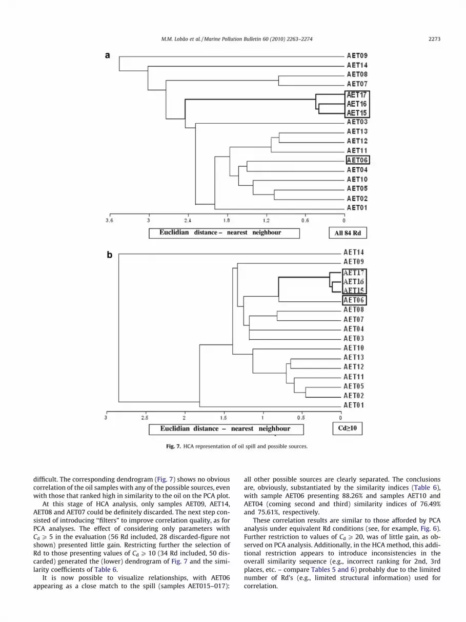
An alternative form of processing and representing the analyti-cal data in this type of correlation study is by Hierarchical ClusterAnalysis (HCA), whose explicit purpose is to organize variables(samples) into clusters, based on their proximity in variable space(Miller and Miller, 2000). The proximity of the groups is usuallypresented in the form of dendrograms, as shown in Fig. 7. Themethod can provide, additionally, a numerical similarity for any
pair of samples from an expression ratioing the distance betweenthe two points of interest and the maximum distance betweenany two points. The exclusion of parameters, as judged convenientfor better correlation quality (e.g., use of ‘‘discrimination capaci-ties”, Cd – as discussed on PCA), can also be introduced.
Similarity (percent) values for the samples are presented in Ta-ble 5. The first HCA plot included, as for PCA, all 84 parameters.Even though sample AET06 shows the highest similarity value(66.81%) with the oil spill (samples AET015, 016 and 017), valuesfor samples AET04 (64.24%) and AET10 (63.22%) are also very highand close to that of sample AET06, making a definite conclusion
Fig. 7. HCA representation of oil spill and possible sources.
difficult. The corresponding dendrogram (Fig. 7) shows no obviouscorrelation of the oil samples with any of the possible sources, evenwith those that ranked high in similarity to the oil on the PCA plot.
At this stage of HCA analysis, only samples AET09, AET14,AET08 and AET07 could be definitely discarded. The next step con-sisted of introducing ‘‘filters” to improve correlation quality, as forPCA analyses. The effect of considering only parameters withCd P 5 in the evaluation (56 Rd included, 28 discarded-figure notshown) presented little gain. Restricting further the selection ofRd to those presenting values of Cd P 10 (34 Rd included, 50 dis-carded) generated the (lower) dendrogram of Fig. 7 and the simi-larity coefficients of Table 6.
It is now possible to visualize relationships, with AET06appearing as a close match to the spill (samples AET015–017):
all other possible sources are clearly separated. The conclusionsare, obviously, substantiated by the similarity indices (Table 6),with sample AET06 presenting 88.26% and samples AET10 andAET04 (coming second and third) similarity indices of 76.49%and 75.61%, respectively.
These correlation results are similar to those afforded by PCAanalysis under equivalent Rd conditions (see, for example, Fig. 6).Further restriction to values of Cd P 20, was of little gain, as ob-served on PCA analysis. Additionally, in the HCA method, this addi-tional restriction appears to introduce inconsistencies in theoverall similarity sequence (e.g., incorrect ranking for 2nd, 3rdplaces, etc. – compare Tables 5 and 6) probably due to the limitednumber of Rd’s (e.g., limited structural information) used forcorrelation.
Table 5HCA similarity indices between spill and suspect sources (all Rd).
The authors thank IEAPM (Navy Research Center) for provisionof oil samples and permission to publish. M.M. Lobao acknowl-edges IEAPM for a leave of absence for his post-graduate studies.
References
Alcantara, E.H., Santos, M.C.F., 2005. XII Annnals of the Brazilian Symposium onRemote Sensing: Mapeamento de áreas de sensibilidade ambiental ao derramede óleo na região portuária de Itaqui, São Luiz, MA-Brasil. INPE, São José dosCampos. p. 4561.
Barakat, A.O., Mostafa, A.R., Rullkötter, J., Hegazi, A.R., 1999. Application of amultimolecular marker approach to fingerprint petroleum in the marineenvironment. Mar. Pollut. Bull. 38, 535–544.
Barakat, A.O., Qian, Y., Kim, M., Kennicutt, M.C., 2001. Chemical characterization ofnaturally weathered oil residues in arid terrestrial environment in Al-Alamein,Egypt, 2001. Environ. Int. 27, 291–310.
Barakat, A.O., Mostafa, A.R., Qian, Y., Kennicutt, M.C., 2002. Application of petroleumchemical fingerprinting in oil spill investigations – Gulf of Suez, Egypt. Spill Sci.Technol. Bull. 7, 229–239.
Boëda, E., Connan, J., Dessort, D., Muhesen, S., Mercier, N., Valladas, H., Tisnérat, N.,1996. Bitumen as a hafting material on Middle Palaeolithic artefacts. Nature380, 336–338.
Bro, R., Sidiropoulos, N.D., Smilde, A.K., 2002. Maximum likelihood fitting ordinaryleast squares algorithms. J. Chemometr. 16, 387–400.
Brown, R.J., 1983. Determination of trace metals in petroleum and petroleumproducts using an inductively-coupled plasma optical emission spectrometer.Spectrochim. Acta B 38, 283–289.
Burns, W.A., Mankiewicz, P.J., Bence, A.E., Page, D.S., Parker, K.R., 1997. A principalcomponent and least-squares method for allocating polycyclic aromatichydrocarbons in sediment to multiple sources. Environ. Toxicol. Chem. 16,119–1131.
Christensen, J.H., Tomasi, G., Hansen, A.B., 2005. Chemical fingerprinting ofpetroleum biomarkers using time warping and PCA. Environ. Sci. Technol. 39,255–260.
Faksness, L.G., Daling, P.S., Hansen, A.B., 2002. Round robin study – oil spillidentification. Environ. Forensics 3, 279–291.
Hosttetler, F.D., Rosenbauer, R.J., Lorenson, T.D., Dougherty, J., 2004. Geochemicalcharacterization of tarballs on beaches along the California coast (part 1).Shallow seepage impacting the Santa Barbara Channel Islands, Santa Cruz, SantaRosa and San Miguel. Org. Geochem. 35, 725–746.
Jeffrey, A.W.A., 2006. Application of stable isotope ratios in spilled oil identification.In: Wang, Z., Stout, S.A. (Eds.), Oil Spill Forensics: Fingerprinting and SourceIdentification. Academic Press, NY, pp. 207–227.
Kennicutt, M.C., 1988. The effect of biodegradation on crude oil bulk and molecularcomposition. Oil Chem. Pollut. 4, 89–112.
Massart, D.L., Vandeginste, B.G.M., Buydens, L.M.C., De Jong, S., Lewi, P.J., Smeyers-Verbeke. J. In Handbook of Chemometrics and Qualimetrics: Part B, vol. 20A,Elsevier, Amsterdam, 1997.
Mello, M.R., Guadalupe, M.D.F., Freitas, L.C.D.S.A., 1990. Proceedings of the 4th.Brazilian Petroleum Conference. Organic Geochemistry applied tocharacterization of oil-spills, Brazilian Petroleum Institute. Rio de Janeiro,Brazil.
Miller, J.C., Miller, J.N., 2000. Statistics and Chemometrics for Analytical Chemistry,4th ed. Prentice Hall, Dorchester, UK.
Murray, A.P., Summons, R.E., Boreham, C.J., Dowling, L.M., 1994. Biomarker and n-alkane isotope profiles for Tertiary oils: relationship to source rock depositionalsetting. Org. Geochem., 521–542.
Peters, K.E., Walters, C.C., Moldowan, J.M., 2005. The Biomarker Guide, 2nd ed.Cambridge University Press, Cambridge, UK.
Shaban, A., Hamze, M., El-Baz, F., Ghoneim, E., 2009. Characterization of an Oil Spillalong the Lebanese Coast by satellite images. Environ. Forensics 10, 51–59.
Stella, A., Piccardo, M.T., Coradeghini, R., Redaelli, A., Lanteri, S., Armanino, C.,Valerio, F., 2002. Principal component analysis application in policyclicaromatic hydrocarbons ‘‘mussel watch” analyses for source identification.Anal. Chim. Acta 461, 201–213.
Stout, S., Uhler, A.D., McCarthy, K.J., 2001. A strategy and methodology fordefensibly correlating spilled oil to source candidates. Environ. Forensics 2,87–98.
Wang, Z.D., Fingas, M., Li, K., 1994. Fractionation of ASMB oil, identification andquantitation of aliphatic, aromatic, and biomarker compounds by GC/FID andGC/MSD (Part I). J. Chromatogr. Sci. 32, 361–366.
Wang, Z., Fingas, M., 1995. Use of methyldibenzothiophenes as markers fordifferentiation and source identification of crude and weathered oils. Environ.Sci. Technol. 29, 2841–2849.
Wang, Z., Fingas, M., Page, D.S., 1999. Oil Spill Identification. J. Chromatogr. A 843,369–411.
Wang, Z., Fingas, M., Sigouin, L., 2002. Using Multiple Criteria for FingerprintingUnknown Oil Samples having very similar chemical composition. Environ.Forensics 3, 251–262.
Wang, Z., Fingas, M., 2003. Development of oil hydrocarbon fingerprinting andidentification techniques. Mar. Pollut. Bull. 47, 423–452.
Wang, Z., Stout, S.A., Fingas, M., 2006. Forensic fingerprinting of biomarkers foroil spill characterization and source identification. Environ. Forensics 7, 105–146.