International Journal of

Environmental Research

and Public Health

Article

Geospatial Distributions of Groundwater Quality inGedaref State Using Geographic Information System(GIS) and Drinking Water Quality Index (DWQI)

Basheer A. Elubid 1,2,* , Tao Huag 1, Ekhlas H. Ahmed 3 , Jianfei Zhao 1, Khalid. M. Elhag 4,Waleed Abbass 2 and Mohammed M. Babiker 5

1 Department of Environmental Science and Engineering, Faculty of Geosciences and EnvironmentalEngineering, Southwest Jiaotong University, high-tech zone, Chengdu 611756, China;basheer@my.swjtu.edu.cn (B.A.E); taohuang70@126.com (T.H.); zhaojianfei@my.swjtu.edu.cn (J.Z.)

2 Department of Hydrogeology, Faculty of Petroleum & Minerals, Al Neelain University, Khartoum 11121,Sudan; elubaid@yahoo.com (B.A.E.); elubbash@hotmail.com (W.A.)

3 School of Resources and Environment, University of Electronic Science and Technology of China,Chengdu 611756, China; 201714180103@std.uestc.edu.cn

4 Key Laboratory of Digital Earth, Institute of Remote Sensing and Digital Earth,Chinese Academy of Sciences, No. 9 Dengzhuang South Road, Haidian District, Beijing 100094, China;khalidelhag@mails.ucas.ac.cn

5 Water Environmental Sanitation Project (WES), Gedaref State Water Corporation, Gedaref 32214, Sudan;ahmed_geonuv@163.com

* Correspondence: basheer@my.swjtu.edu.cn or elubaid@yahoo.com; Tel.: +86-152-0821-4309 or +86-173-0809-4289

Received: 4 December 2018; Accepted: 17 February 2019; Published: 28 February 2019�����������������

Abstract: The observation of groundwater quality elements is essential for understanding theclassification and distribution of drinking water. Geographic Information System (GIS) and remotesensing (RS), are intensive tools for the performance and analysis of spatial datum associated withgroundwater sources control. In this study, groundwater quality parameters were observed in threedifferent aquifers including: sandstone, alluvium and basalt. These aquifers are the primary sourceof national drinking water and partly for agricultural activity in El Faw, El Raha (Fw-Rh), El Qalabatand El Quresha (Qa-Qu) localities in the southern part of Gedaref State in eastern Sudan. The aquifershave been overworked intensively as the main source of indigenous water supply in the study area.The interpolation methods were used to demonstrate the facies pattern and Drinking Water QualityIndex (DWQI) of the groundwater in the research area. The GIS interpolation tool was used to obtainthe spatial distribution of groundwater quality parameters and DWQI in the area. Forty sampleswere assembled and investigated for the analysis of major cations and anions. The groundwaterin this research is controlled by sodium and bicarbonate ions that defined the composition of thewater type to be Na HCO3. However, from the plots of piper diagram; the samples result revealed(40%) Na-Mg-HCO3 and (35%) Na-HCO3 water types. The outcome of the analysis reveals thatseveral groundwater samples have been found to be suitable for drinking purposes in Fa-Rh andQa-Qu areas.

Keywords: aquifers; drinking water quality index DWQI; spatial distribution; piper diagram;interpolation methods

1. Introduction

Groundwater is a noble resource for water in arid and semiarid areas [1–6]. Accessibility to wateris an important global goal whose effects are abundantly felt in developing countries. The benefit of

Int. J. Environ. Res. Public Health 2019, 16, 731; doi:10.3390/ijerph16050731 www.mdpi.com/journal/ijerph

Int. J. Environ. Res. Public Health 2019, 16, 731 2 of 20

understanding groundwater geochemistry is to ensure its good quality for drinking [7–9]. In arid andsemi-arid areas, the potential use of groundwater for drinking and agricultural projects is threatenedby the decline of water quality due to physical and anthropogenic characteristics. Evaluation of thegeochemical status of groundwater is required to competently plan and control the groundwaterresources [10]. The interaction between water and rocks has usually been studied to providean understanding of the physical and chemical procedures controlling water chemistry [11–13].Several factors control the groundwater geochemistry such as the type of rock forming the aquifer,the residence time of water in the hosted aquifer, the origin of the groundwater and the flow directionsof groundwater [14,15].

The estimation of quality and the use of groundwater for different purposes are becomingmore significant [16]. Thus, probes related to an understanding of the hydro-chemical aspects ofthe groundwater, geochemical processes and its development under natural water flowing manners,not only aids in the practical utilization and protection of this expensive resource but also aid invisualizing the changes in the groundwater environment [17,18].

Statistical analysis methods such as the correlation matrix, bivariate, and Hierarchal componentanalysis; produce a reliable alternative procedure for understanding and explaining the complexsystem of water quality with the capability of analyzing large amounts of data [19].

GIS and RS, are intensive tools for performance and analysis of spatial datum associated withgroundwater sources control. Remote sensing data are essential in many geo-resources, such asmineral research, hydrogeology, and other geologic fields [20]. It is important in hydrogeologicalreconnaissance for understanding structural, geomorphological, and lithological features. The acquiredRS information improves our knowledge of the hydrogeological conditions. Satellite images areuniversally applied for qualitative estimation of groundwater resources by investigating geologicalstructures, geomorphic features, and their hydrological characteristics [21–23]. The spatial distributionmaps were designed and integrated within ArcGIS v.10.5 software.

Drinking water quality index (DWQI) presents a single number to reveal the overall waterquality at a particular position and time, based on various water quality factors. It is interpretedas a number that indicates the combined impact of several water quality parameters [19,24–28].DWQI has been popularly utilized in water quality evaluations for both surface and sub-surface water,and it has represented an increasingly significant function in the water resource environment andmanagement [29–31].

Shortage of drinking water in East Central Sudan especially in the basaltic terrain is a commonproblem. Most of the rural community depends on groundwater sources in their daily life for drinkingpurposes. This research aims to generate groundwater distribution maps and to evaluate water qualityfor drinking purposes in Qa-Qu and Fw-Rh areas in the southern part of Gedaref State in easternSudan. The area consists of one of the essential agricultural fields of Gedaref State, the El Rahad projectwhich was developed as a mechanized project in Sudan in 1978 [32].

In this work, forty samples were observed and monitored from selected boreholes.Hence, an attempt of statistical analysis methods such as correlation matrix and Hierarchal componentanalysis were applied to determine the variation in hydro-chemical facies and understand thedevelopment of hydro-chemical processes. Moreover, adopting Piper and Durov diagrams by useof Aqua Chem. v.2014.2 software, to classify the groundwater facies and water types in the area.The world health organization (WHO) [33] standard has been used for correlations with the results ofsample analysis to examine the permissible amount of water for drinking.

The analytical results achieved from the samples when plotted on Piper’s plot, explained that thealkalis (Na+, K+), appear considerably over the alkaline elements (Ca2+, Mg2+), and the weak acidic(HCO3

−) appear considerably over strong acidic anions (Cl− & SO4−2). Moreover, the Piper diagram

matched 40% of the samples, under Na-Mg-HCO3 group and 35% under Na-HCO3 type. According tothe plotting from the Durov diagram, most of the elements of water plotted within the HCO3·Nazone, except some other samples that fell in HCO3 Cl-Na, SO4·Cl·HCO3-Na, or HCO3·Cl-Na·Mg types.

Int. J. Environ. Res. Public Health 2019, 16, 731 3 of 20

DWQI was calculated by adopting weighted arithmetical index methods considering thirteen waterquality parameters (pH, TDS, Ca+2, Mg+2, Na+, K+, Fe+2, Cl−, HCO3

−, SO4−2, F−, NO3

−, and E.C) inorder to assess the degree of groundwater contamination and suitability for drinking purposes.

For the better understanding of geological units in this project, the thin sections of rock sampleshave been generated. With this ability, the rock mineral contents have been determined much better.This study has great importance; due to the plan for obtaining drinking water from the groundwatersources to Fw-Rh and Qa-Qu localities. However, this investigation is helpful in understandinggroundwater environments and its suitability for human uses, especially in arid and semi-arid regions.

2. Materials and Methods

2.1. Geology

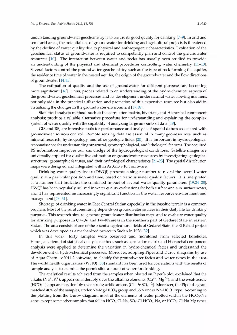
Geologically Figure 1; the lower Proterozoic rocks of the basement complex (Mainly GraniticGneisses) [34], Syn-orogenic Granit and Syn-orogenic gabbro underlain the sandstone of Gedaref formation,Tertiary (Oligocene) basalt [35], Umm Rawaba formation, sand sheets and recent alluvium and wadi deposits.The groundwater of the area was taped at the sandstone of Gedaref formation sequence, alluvium soil,and fractures of the Oligocene basalt aquifers with depths ranging from 14 to 64 m.

Int. J. Environ. Res. Public Health 2019, 16, x FOR PEER REVIEW 3 of 19

DWQI was calculated by adopting weighted arithmetical index methods considering thirteen water quality parameters (pH, TDS, Ca+2, Mg+2, Na+, K+, Fe+2, Cl−, HCO3−, SO4−2, F−, NO3−, and E.C) in order to assess the degree of groundwater contamination and suitability for drinking purposes.

For the better understanding of geological units in this project, the thin sections of rock samples have been generated. With this ability, the rock mineral contents have been determined much better. This study has great importance; due to the plan for obtaining drinking water from the groundwater sources to Fw-Rh and Qa-Qu localities. However, this investigation is helpful in understanding groundwater environments and its suitability for human uses, especially in arid and semi-arid regions.

2. Materials and Methods

2.1. Geology

Geologically Figure 1; the lower Proterozoic rocks of the basement complex (Mainly Granitic Gneisses) [34], Syn-orogenic Granit and Syn-orogenic gabbro underlain the sandstone of Gedaref formation, Tertiary (Oligocene) basalt [35], Umm Rawaba formation, sand sheets and recent alluvium and wadi deposits. The groundwater of the area was taped at the sandstone of Gedaref formation sequence, alluvium soil, and fractures of the Oligocene basalt aquifers with depths ranging from 14 to 64 m.

Figure 1. Location map and geological units of study area.

2.2. Hydrogeological Setting

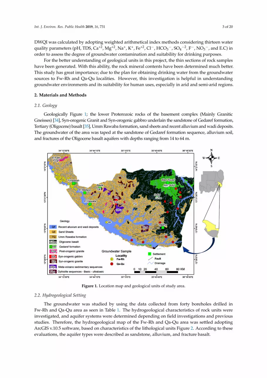
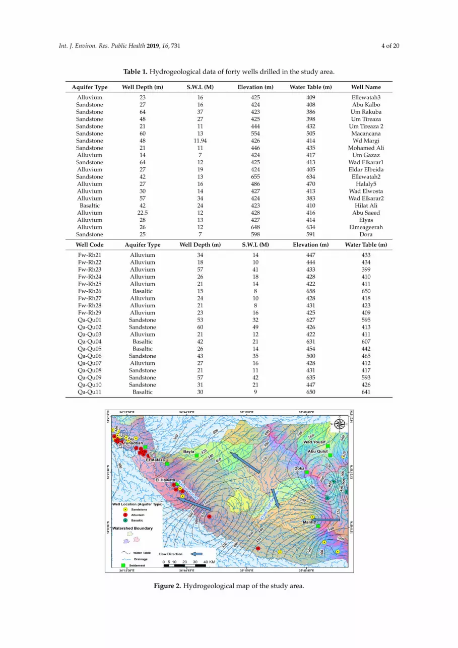
The groundwater was studied by using the data collected from forty boreholes drilled in Fw-Rh and Qa-Qu area as seen in Table 1. The hydrogeological characteristics of rock units were investigated, and aquifer systems were determined depending on field investigations and previous studies. Therefore, the hydrogeological map of the Fw-Rh and Qa-Qu area was settled adopting ArcGIS v.10.5 software, based on characteristics of the lithological units Figure 2. According to these evaluations, the aquifer types were described as sandstone, alluvium, and fracture basalt.

Figure 1. Location map and geological units of study area.

2.2. Hydrogeological Setting

The groundwater was studied by using the data collected from forty boreholes drilled inFw-Rh and Qa-Qu area as seen in Table 1. The hydrogeological characteristics of rock units wereinvestigated, and aquifer systems were determined depending on field investigations and previousstudies. Therefore, the hydrogeological map of the Fw-Rh and Qa-Qu area was settled adoptingArcGIS v.10.5 software, based on characteristics of the lithological units Figure 2. According to theseevaluations, the aquifer types were described as sandstone, alluvium, and fracture basalt.

Int. J. Environ. Res. Public Health 2019, 16, 731 4 of 20

Table 1. Hydrogeological data of forty wells drilled in the study area.

Aquifer Type Well Depth (m) S.W.L (M) Elevation (m) Water Table (m) Well Name

Alluvium 23 16 425 409 Ellewatah3Sandstone 27 16 424 408 Abu KalboSandstone 64 37 423 386 Um RakubaSandstone 48 27 425 398 Um TireazaSandstone 21 11 444 432 Um Tireaza 2Sandstone 60 13 554 505 MacancanaSandstone 48 11.94 426 414 Wd MargiSandstone 21 11 446 435 Mohamed AliAlluvium 14 7 424 417 Um GazazSandstone 64 12 425 413 Wad Elkarar1Alluvium 27 19 424 405 Eldar ElbeidaSandstone 42 13 655 634 Ellewatah2Alluvium 27 16 486 470 Halaly5Alluvium 30 14 427 413 Wad ElwostaAlluvium 57 34 424 383 Wad Elkarar2Basaltic 42 24 423 410 Hilat Ali

Alluvium 22.5 12 428 416 Abu SaeedAlluvium 28 13 427 414 ElyasAlluvium 26 12 648 634 ElmeageerahSandstone 25 7 598 591 Dora

Well Code Aquifer Type Well Depth (m) S.W.L (M) Elevation (m) Water Table (m)

Fw-Rh21 Alluvium 34 14 447 433Fw-Rh22 Alluvium 18 10 444 434Fw-Rh23 Alluvium 57 41 433 399Fw-Rh24 Alluvium 26 18 428 410Fw-Rh25 Alluvium 21 14 422 411Fw-Rh26 Basaltic 15 8 658 650Fw-Rh27 Alluvium 24 10 428 418Fw-Rh28 Alluvium 21 8 431 423Fw-Rh29 Alluvium 23 16 425 409Qa-Qu01 Sandstone 53 32 627 595Qa-Qu02 Sandstone 60 49 426 413Qa-Qu03 Alluvium 21 12 422 411Qa-Qu04 Basaltic 42 21 631 607Qa-Qu05 Basaltic 26 14 454 442Qa-Qu06 Sandstone 43 35 500 465Qa-Qu07 Alluvium 27 16 428 412Qa-Qu08 Sandstone 21 11 431 417Qa-Qu09 Sandstone 57 42 635 593Qa-Qu10 Sandstone 31 21 447 426Qa-Qu11 Basaltic 30 9 650 641

Int. J. Environ. Res. Public Health 2019, 16, x FOR PEER REVIEW 4 of 19

Table 1. Hydrogeological data of forty wells drilled in the study area.

Aquifer Type Well Depth (m) S.W.L (M) Elevation (m) Water Table (m) Well Name Alluvium 23 16 425 409 Ellewatah3 Sandstone 27 16 424 408 Abu Kalbo Sandstone 64 37 423 386 Um Rakuba Sandstone 48 27 425 398 Um Tireaza Sandstone 21 11 444 432 Um Tireaza 2 Sandstone 60 13 554 505 Macancana Sandstone 48 11.94 426 414 Wd Margi Sandstone 21 11 446 435 Mohamed Ali Alluvium 14 7 424 417 Um Gazaz Sandstone 64 12 425 413 Wad Elkarar1 Alluvium 27 19 424 405 Eldar Elbeida Sandstone 42 13 655 634 Ellewatah2 Alluvium 27 16 486 470 Halaly5 Alluvium 30 14 427 413 Wad Elwosta Alluvium 57 34 424 383 Wad Elkarar2 Basaltic 42 24 423 410 Hilat Ali

Alluvium 22.5 12 428 416 Abu Saeed Alluvium 28 13 427 414 Elyas Alluvium 26 12 648 634 Elmeageerah Sandstone 25 7 598 591 Dora Well Code Aquifer Type Well Depth (m) S.W.L (M) Elevation (m) Water Table (m) Fw-Rh21 Alluvium 34 14 447 433 Fw-Rh22 Alluvium 18 10 444 434 Fw-Rh23 Alluvium 57 41 433 399 Fw-Rh24 Alluvium 26 18 428 410 Fw-Rh25 Alluvium 21 14 422 411 Fw-Rh26 Basaltic 15 8 658 650 Fw-Rh27 Alluvium 24 10 428 418 Fw-Rh28 Alluvium 21 8 431 423 Fw-Rh29 Alluvium 23 16 425 409 Qa-Qu01 Sandstone 53 32 627 595 Qa-Qu02 Sandstone 60 49 426 413 Qa-Qu03 Alluvium 21 12 422 411 Qa-Qu04 Basaltic 42 21 631 607 Qa-Qu05 Basaltic 26 14 454 442 Qa-Qu06 Sandstone 43 35 500 465 Qa-Qu07 Alluvium 27 16 428 412 Qa-Qu08 Sandstone 21 11 431 417 Qa-Qu09 Sandstone 57 42 635 593 Qa-Qu10 Sandstone 31 21 447 426 Qa-Qu11 Basaltic 30 9 650 641

Figure 2. Hydrogeological map of the study area. Figure 2. Hydrogeological map of the study area.

Int. J. Environ. Res. Public Health 2019, 16, 731 5 of 20

2.3. Spatial Interpolation and Groundwater Quality Mapping

Spatial interpolation is a procedure of predicting the value of attributes at unsampled sites frommeasurements made at point locations within the same area [36]. There are two main groupings ofinterpolation techniques: deterministic and geostatistical. Deterministic interpolation techniques createsurfaces from measured points, based on either the extent of similarity (e.g., Inverse Distance Weighted)or the degree of smoothing (e.g., radial basis functions). Geostatistical interpolation techniques(e.g., kriging) utilize the statistical properties of the measured points.

In this study, we found that the Kriging (Ordinary and Simple) interpolation method is the mostsuitable method. Thus, the histograms and normal QQplots were plotted to examine the normalitydistribution of the observed data for each water quality element in both Fw-Rh and Qa-Qu localities.

2.4. Drinking Water Quality Index DWQI

DWQI has been determined based on the standards of drinking water quality as counseledby WHO. Therefore, thirteen chemical parameters (pH, TDS, Ca, Mg, Na, K, Cl, HCO3, F, NO3, Fe,and E.C.) were used for the calculation. To apply DWQI in the current study, the study area wasdivided into two parts, Fw-Rh, and Qa-Qu localities. The water quality parts were generated bya weighting factor and then formerly aggregated by using the simple mean calculations. To estimatethe water quality in this project, the quality rating (Qi) for all elements was estimated through thefollowing equation;

Qi = {(Va −Vi/Vs −Vi)} ∗ 100 (1)

where, Qi = Quality ranking of the element form a total number of water quality elements, Va = Realamount of the water quality element taken from laboratory study, Vi = Ideal rate of the water qualityelement can be realized from the standard Tables. Vi for pH = 7 and for other elements it is equaling tozero. Vs standard = Value of WHO standard.

Then, the Relative weight (Wr) was studied from inversed proportional of recommended standard(Si) for the corresponding parameter using the following expression;

Wr =I

Si(2)

Here Wr = Relative (unit) weight for specific element; Si = Standard allowable amount for certainelement; I = Proportionality constant.

Assuredly, the total DWQI was determined using the assemblage equations of the quality ratingwith the unit weight linearly as the following:

DWQI = ∑ QiWr/ ∑ Wr# (3)

where Qi = Quality rating; Wr = Relative weight.In general, DWQI is determined for particular and intended uses of water. In this work, the DWQI

was estimated for human consumption, and the maximum DWQI value for the drinking purposes wasregarded as 100 scores.

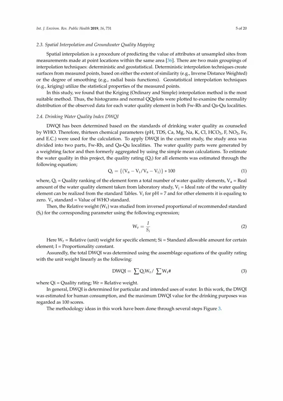
The methodology ideas in this work have been done through several steps Figure 3.

Int. J. Environ. Res. Public Health 2019, 16, 731 6 of 20

Int. J. Environ. Res. Public Health 2019, 16, x FOR PEER REVIEW 6 of 19

Figure 3. Methodology chart of study procedures.

3. Results

Several factors may control the groundwater geochemistry such as the type of rock forming the aquifer, residence time of water in the hosted aquifer, the origin of the groundwater and the flow directions of groundwater. Hydro-chemical properties of the groundwater of the area are shown in Table 2. The water pH ranges between 7.5 and 8.9, indicate an alkaline chemical reaction in both sandstone and basaltic aquifers. The electrical conductivity (E.C) varies from 345 to 3342 μS/cm.

Table 2. Descriptive statistical analysis result of water samples (N = 40).

Fw-Rh (N = 29) Qa-Qu (N = 11) Variable WHO Minimum Maximum Mean Std. D. Minimum Maximum Mean Std. D.

pH 7.0–8.0 7.50 8.90 8.03 0.35 7.60 8.70 7.96 0.32 TDS (mg/L) 1000 242.00 2340.00 601.72 399.60 183.00 2007.00 663.18 502.41

Ca 75 4.45 130.00 37.47 30.06 10.44 53.00 22.21 12.43 Mg 30 11.66 120.53 34.28 23.86 11.56 72.00 36.20 18.23 Na 200 76.00 359.00 214.28 69.87 76.00 597.00 167.18 150.29 K - 15.00 70.00 41.72 13.40 16.00 115.00 33.36 28.68 Cl 250 8.10 172.50 35.90 37.69 10.00 45.00 21.39 8.96

HCO3 - 78.90 1450.00 499.35 311.78 118.60 930.00 355.40 247.40 SO4 250 0.02 2.57 0.74 0.70 1.36 2.29 1.83 0.31

F 0.5–1 0.01 2.56 0.55 0.55 0.02 2.56 0.65 0.70 NO3 50 0.20 15.00 3.88 3.96 1.50 11.10 5.05 3.11 Fe 0.03 0.01 0.80 0.15 0.22 0.01 1.04 0.19 0.31

E.C (μ.S/cm)

- 345.00 3342.00 888.23 570.54 281.53 9692.00 1777.97 2721.19

(WHO)= The world health organization standard

3.1. Interpolation and Elements Distribution Maps

The quality of interpolation is described by the difference of the interpolated value from the true value. Thus, the Anderson-Darling test, which is an ECDF (empirical cumulative distribution function) based test, tests the prospect that the value of a parameter falls within a particular range of values (confidence level 95%). The data points are relatively close to the fitted normal distribution line. The p-value is greater than the significance level of 0.05. Subsequently, the scientist fails to reject the null hypothesis that the data follow a normal distribution.

Figure 3. Methodology chart of study procedures.

3. Results

Several factors may control the groundwater geochemistry such as the type of rock forming theaquifer, residence time of water in the hosted aquifer, the origin of the groundwater and the flowdirections of groundwater. Hydro-chemical properties of the groundwater of the area are shown inTable 2. The water pH ranges between 7.5 and 8.9, indicate an alkaline chemical reaction in bothsandstone and basaltic aquifers. The electrical conductivity (E.C) varies from 345 to 3342 µS/cm.

Table 2. Descriptive statistical analysis result of water samples (N = 40).

Fw-Rh (N = 29) Qa-Qu (N = 11)

Variable WHO Minimum Maximum Mean Std. D. Minimum Maximum Mean Std. D.

pH 7.0–8.0 7.50 8.90 8.03 0.35 7.60 8.70 7.96 0.32TDS (mg/L) 1000 242.00 2340.00 601.72 399.60 183.00 2007.00 663.18 502.41

Ca 75 4.45 130.00 37.47 30.06 10.44 53.00 22.21 12.43Mg 30 11.66 120.53 34.28 23.86 11.56 72.00 36.20 18.23Na 200 76.00 359.00 214.28 69.87 76.00 597.00 167.18 150.29K - 15.00 70.00 41.72 13.40 16.00 115.00 33.36 28.68Cl 250 8.10 172.50 35.90 37.69 10.00 45.00 21.39 8.96

HCO3 - 78.90 1450.00 499.35 311.78 118.60 930.00 355.40 247.40SO4 250 0.02 2.57 0.74 0.70 1.36 2.29 1.83 0.31

F 0.5–1 0.01 2.56 0.55 0.55 0.02 2.56 0.65 0.70NO3 50 0.20 15.00 3.88 3.96 1.50 11.10 5.05 3.11

Fe 0.03 0.01 0.80 0.15 0.22 0.01 1.04 0.19 0.31E.C (µ.S/cm) - 345.00 3342.00 888.23 570.54 281.53 9692.00 1777.97 2721.19

(WHO)= The world health organization standard.

3.1. Interpolation and Elements Distribution Maps

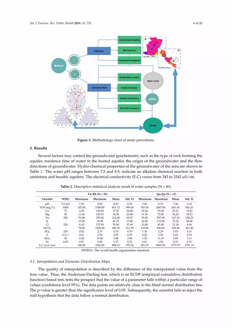
The quality of interpolation is described by the difference of the interpolated value from thetrue value. Thus, the Anderson-Darling test, which is an ECDF (empirical cumulative distributionfunction) based test, tests the prospect that the value of a parameter falls within a particular range ofvalues (confidence level 95%). The data points are relatively close to the fitted normal distribution line.The p-value is greater than the significance level of 0.05. Subsequently, the scientist fails to reject thenull hypothesis that the data follow a normal distribution.

Int. J. Environ. Res. Public Health 2019, 16, 731 7 of 20

According to this test, in Fw-Rh area we found that the parameters (Na and K) showed a normaldistribution when the other elements (Ca, Mg, HCO3, Cl, SO4 and TDS) showed a more or lessabnormal distribution in Figures 4 and 5.

Int. J. Environ. Res. Public Health 2019, 16, x FOR PEER REVIEW 7 of 19

According to this test, in Fw-Rh area we found that the parameters (Na and K) showed a normal distribution when the other elements (Ca, Mg, HCO3, Cl, SO4 and TDS) showed a more or less abnormal distribution in Figures 4 and 5.

Figure 4. Graphical summary and probability plots of cations in Fw-Rh area. Figure 4. Graphical summary and probability plots of cations in Fw-Rh area.

Int. J. Environ. Res. Public Health 2019, 16, 731 8 of 20Int. J. Environ. Res. Public Health 2019, 16, x FOR PEER REVIEW 8 of 19

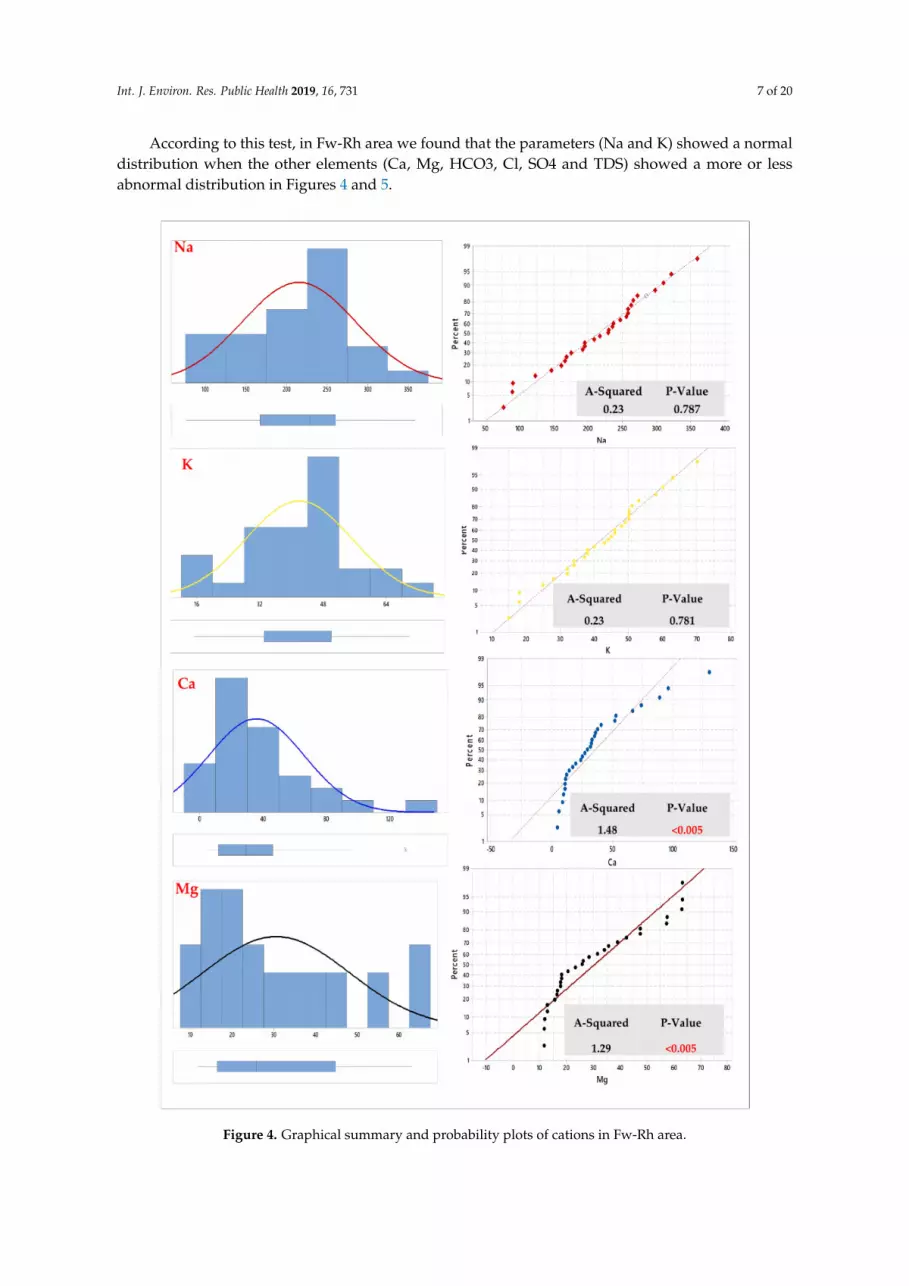
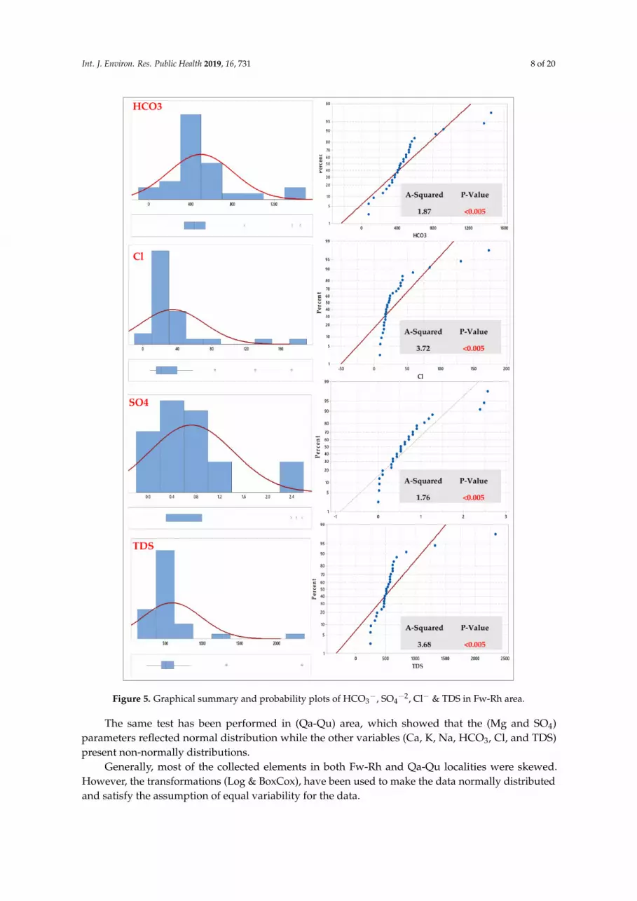
Figure 5. Graphical summary and probability plots of HCO3−, SO4−2, Cl− & TDS in Fw-Rh area.

The same test has been performed in (Qa-Qu) area, which showed that the (Mg and SO4) parameters reflected normal distribution while the other variables (Ca, K, Na, HCO3, Cl, and TDS) present non-normally distributions.

Generally, most of the collected elements in both Fw-Rh and Qa-Qu localities were skewed. However, the transformations (Log & BoxCox), have been used to make the data normally distributed and satisfy the assumption of equal variability for the data.

For the maps prediction, several kinds of semivariogram models were examined for each water quality parameter to obtain the preferable one, as seen in Figure 6 as an example. Predictive performances of the fitted models were checked on the basis of cross-validation tests. The values of

Figure 5. Graphical summary and probability plots of HCO3−, SO4

−2, Cl− & TDS in Fw-Rh area.

The same test has been performed in (Qa-Qu) area, which showed that the (Mg and SO4)parameters reflected normal distribution while the other variables (Ca, K, Na, HCO3, Cl, and TDS)present non-normally distributions.

Generally, most of the collected elements in both Fw-Rh and Qa-Qu localities were skewed.However, the transformations (Log & BoxCox), have been used to make the data normally distributedand satisfy the assumption of equal variability for the data.

Int. J. Environ. Res. Public Health 2019, 16, 731 9 of 20

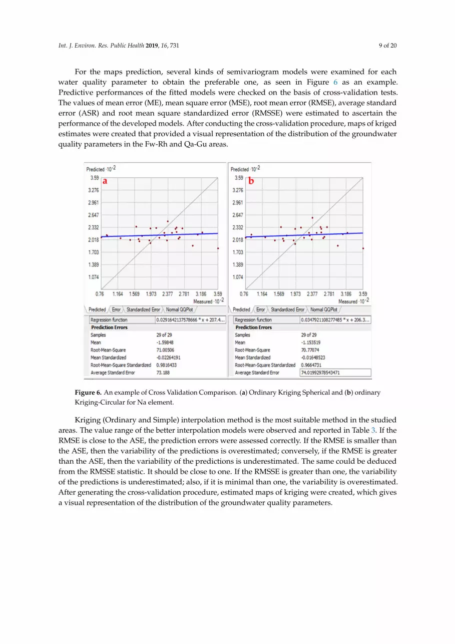
For the maps prediction, several kinds of semivariogram models were examined for eachwater quality parameter to obtain the preferable one, as seen in Figure 6 as an example.Predictive performances of the fitted models were checked on the basis of cross-validation tests.The values of mean error (ME), mean square error (MSE), root mean error (RMSE), average standarderror (ASR) and root mean square standardized error (RMSSE) were estimated to ascertain theperformance of the developed models. After conducting the cross-validation procedure, maps of krigedestimates were created that provided a visual representation of the distribution of the groundwaterquality parameters in the Fw-Rh and Qa-Gu areas.

Int. J. Environ. Res. Public Health 2019, 16, x FOR PEER REVIEW 9 of 19

mean error (ME), mean square error (MSE), root mean error (RMSE), average standard error (ASR) and root mean square standardized error (RMSSE) were estimated to ascertain the performance of the developed models. After conducting the cross-validation procedure, maps of kriged estimates were created that provided a visual representation of the distribution of the groundwater quality parameters in the Fw-Rh and Qa-Gu areas.

Figure 6. An example of Cross Validation Comparison. (a) Ordinary Kriging Spherical and (b) ordinary Kriging-Circular for Na element.

Kriging (Ordinary and Simple) interpolation method is the most suitable method in the studied areas. The value range of the better interpolation models were observed and reported in Table 3. If the RMSE is close to the ASE, the prediction errors were assessed correctly. If the RMSE is smaller than the ASE, then the variability of the predictions is overestimated; conversely, if the RMSE is greater than the ASE, then the variability of the predictions is underestimated. The same could be deduced from the RMSSE statistic. It should be close to one. If the RMSSE is greater than one, the variability of the predictions is underestimated; also, if it is minimal than one, the variability is overestimated. After generating the cross-validation procedure, estimated maps of kriging were created, which gives a visual representation of the distribution of the groundwater quality parameters.

Table 3. Characteristics parameters of variogram models.

Area Groundwater

Parameters Kriging

Type Transformation

Best Fitted Model

ME RMSE ASE MSE RMSSE

Fw-Rh

Na Simple None Spherical −1.5985 71.0051 73.1880 −0.0226 0.9816 K Ordinary None Spherical −0.2818 13.6108 14.0445 −0.0207 0.9817 Ca Ordinary Log Circular 0.6579 32.1486 30.1062 0.0155 1.0624 Mg Ordinary Log Gaussian 0.5210 18.9853 22.6372 −0.0224 0.8808

HCO3 Ordinary BoxCox Stable 19.5080 328.5189 367.5360 0.0498 0.9083 Cl Ordinary Log Circular −0.4151 38.0299 37.4075 −0.0077 1.0432

SO4 Ordinary BoxCox Stable 0.0593 0.6693 0.6351 0.0892 1.0814 TDS Ordinary BoxCox Stable 12.4257 434.6693 453.4310 0.0294 1.0040

Qa-Q

u

Na Simple None Stable 10.9458 143.4509 156.6227 0.0688 0.8907 K Simple Log Spherical −0.1683 27.1142 19.2757 −0.0102 1.4215 Ca Simple BoxCox Stable −0.3761 14.1042 11.5697 −0.0176 1.1645 Mg Ordinary Log Circular 1.6593 20.6180 23.8640 −0.0615 1.0218

HCO3 Ordinary BoxCox Stable 15.3778 261.7170 258.9817 0.0556 0.9939 Cl Ordinary Log Stable −0.3736 9.6335 7.1223 −0.1165 1.2648

SO4 Ordinary None Spherical 0.0251 0.3209 0.3193 0.0654 1.0026 TDS Simple BoxCox Gaussian 6.7649 614.1923 453.6139 −0.2829 1.8464

(ME)= Values of mean error, (RMSE)= Root mean error, (ASE)= Average standard error, (MSE)= Mean square error, (RMSSE)= Root mean square standardized error.

Figure 6. An example of Cross Validation Comparison. (a) Ordinary Kriging Spherical and (b) ordinaryKriging-Circular for Na element.

Kriging (Ordinary and Simple) interpolation method is the most suitable method in the studiedareas. The value range of the better interpolation models were observed and reported in Table 3. If theRMSE is close to the ASE, the prediction errors were assessed correctly. If the RMSE is smaller thanthe ASE, then the variability of the predictions is overestimated; conversely, if the RMSE is greaterthan the ASE, then the variability of the predictions is underestimated. The same could be deducedfrom the RMSSE statistic. It should be close to one. If the RMSSE is greater than one, the variabilityof the predictions is underestimated; also, if it is minimal than one, the variability is overestimated.After generating the cross-validation procedure, estimated maps of kriging were created, which givesa visual representation of the distribution of the groundwater quality parameters.

Int. J. Environ. Res. Public Health 2019, 16, 731 10 of 20

Table 3. Characteristics parameters of variogram models.

Area GroundwaterParameters

KrigingType Transformation Best Fitted

Model ME RMSE ASE MSE RMSSE

Fw-R

h

Na Simple None Spherical −1.5985 71.0051 73.1880 −0.0226 0.9816K Ordinary None Spherical −0.2818 13.6108 14.0445 −0.0207 0.9817Ca Ordinary Log Circular 0.6579 32.1486 30.1062 0.0155 1.0624Mg Ordinary Log Gaussian 0.5210 18.9853 22.6372 −0.0224 0.8808

HCO3 Ordinary BoxCox Stable 19.5080 328.5189 367.5360 0.0498 0.9083Cl Ordinary Log Circular −0.4151 38.0299 37.4075 −0.0077 1.0432

SO4 Ordinary BoxCox Stable 0.0593 0.6693 0.6351 0.0892 1.0814TDS Ordinary BoxCox Stable 12.4257 434.6693 453.4310 0.0294 1.0040

Qa-

Qu

Na Simple None Stable 10.9458 143.4509 156.6227 0.0688 0.8907K Simple Log Spherical −0.1683 27.1142 19.2757 −0.0102 1.4215Ca Simple BoxCox Stable −0.3761 14.1042 11.5697 −0.0176 1.1645Mg Ordinary Log Circular 1.6593 20.6180 23.8640 −0.0615 1.0218

HCO3 Ordinary BoxCox Stable 15.3778 261.7170 258.9817 0.0556 0.9939Cl Ordinary Log Stable −0.3736 9.6335 7.1223 −0.1165 1.2648

SO4 Ordinary None Spherical 0.0251 0.3209 0.3193 0.0654 1.0026TDS Simple BoxCox Gaussian 6.7649 614.1923 453.6139 −0.2829 1.8464

(ME)= Values of mean error, (RMSE)= Root mean error, (ASE)= Average standard error, (MSE)= Mean square error,(RMSSE)= Root mean square standardized error.

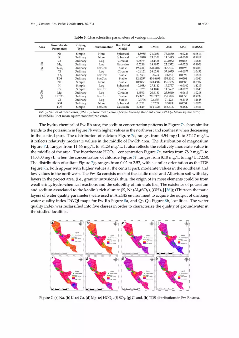
The hydro-chemical of Fw-Rh area; the sodium concentration patterns in Figure 7a show similartrends to the potassium in Figure 7b with higher values in the northwest and southeast when decreasingin the central part. The distribution of calcium Figure 7c, ranges from 4.54 mg/L to 37.47 mg/L,it reflects relatively moderate values in the middle of Fw-Rh area. The distribution of magnesiumFigure 7d, ranges from 11.66 mg/L to 34.28 mg/L. It also reflects the relatively moderate value inthe middle of the area. The bicarbonate HCO3

− concentration Figure 7e, varies from 78.9 mg/L to1450.00 mg/L, when the concentration of chloride Figure 7f, ranges from 8.10 mg/L to mg/L 172.50.The distribution of sulfate Figure 7g, ranges from 0.02 to 2.57, with a similar orientation as the TDSFigure 7h, both appear with higher values at the central part, moderate values in the southeast andlow values in the northwest. The Fw-Ra consists most of the acidic rocks and Alluvium soil with claylayers in the project area, (i.e., granitic intrusions), thus, the origin of its most elements could be fromweathering, hydro-chemical reactions and the solubility of minerals (i.e., The existence of potassiumand sodium associated to the kaolin’s rich alunite (K, Na)Al3(SO4)2(OH)6] [36]); (Thirteen thematiclayers of water quality parameters were used in ArcGIS environment to acquire the output of drinkingwater quality index DWQI maps for Fw-Rh Figure 8a, and Qa-Qu Figure 8b, localities. The waterquality index was reclassified into five classes in order to characterize the quality of groundwater inthe studied localities.

Int. J. Environ. Res. Public Health 2019, 16, x FOR PEER REVIEW 10 of 19

The hydro-chemical of Fw-Rh area; the sodium concentration patterns in Figure 7a show similar trends to the potassium in Figure 7b with higher values in the northwest and southeast when decreasing in the central part. The distribution of calcium Figure 7c, ranges from 4.54 mg/L to 37.47 mg/L, it reflects relatively moderate values in the middle of Fw-Rh area. The distribution of magnesium Figure 7d, ranges from 11.66 mg/L to 34.28 mg/L. It also reflects the relatively moderate value in the middle of the area. The bicarbonate HCO3− concentration Figure 7e, varies from 78.9 mg/L to 1450.00 mg/L, when the concentration of chloride Figure 7f, ranges from 8.10 mg/L to mg/L 172.50. The distribution of sulfate Figure 7g, ranges from 0.02 to 2.57, with a similar orientation as the TDS Figure 7h, both appear with higher values at the central part, moderate values in the southeast and low values in the northwest. The Fw-Ra consists most of the acidic rocks and Alluvium soil with clay layers in the project area, (i.e., granitic intrusions), thus, the origin of its most elements could be from weathering, hydro-chemical reactions and the solubility of minerals (i.e., The existence of potassium and sodium associated to the kaolin’s rich alunite (K, Na)Al3(SO4)2(OH)6] [37]); (Thirteen thematic layers of water quality parameters were used in ArcGIS environment to acquire the output of drinking water quality index DWQI maps for Fw-Rh Figure 8a, and Qa-Qu Figure 8b, localities. The water quality index was reclassified into five classes in order to characterize the quality of groundwater in the studied localities.

Figure 7. (a) Na, (b) K, (c) Ca, (d) Mg, (e) HCO3, (f) SO4, (g) Cl and, (h) TDS distributions in Fw-Rh area.

Figure 8 Spatial interpolation of Drinking Water Quality Index (DWQI). (a) Fw-Rh and (b) Qa-Qu localities Discussion.

The hydro-chemical of Qa-Qu area; the sodium concentration in Figure 9a has similar trends as the potassium Figure 9b, with higher values in the east, middle values in the northwest to the north and low values in the southern part. The distribution of calcium in Figure 9c, ranges from 10.44 mg/L to 53.00 mg/L, the high values concentrated in the middle of Qa-Qu area, then decreases gradually to the north and south. The magnesium Figure 9d, ranges from 11.56 mg/L to 72.00 mg/L. It reflects

Figure 7. (a) Na, (b) K, (c) Ca, (d) Mg, (e) HCO3, (f) SO4, (g) Cl and, (h) TDS distributions in Fw-Rh area.

Int. J. Environ. Res. Public Health 2019, 16, 731 11 of 20

Int. J. Environ. Res. Public Health 2019, 16, x FOR PEER REVIEW 10 of 19

The hydro-chemical of Fw-Rh area; the sodium concentration patterns in Figure 7a show similar trends to the potassium in Figure 7b with higher values in the northwest and southeast when decreasing in the central part. The distribution of calcium Figure 7c, ranges from 4.54 mg/L to 37.47 mg/L, it reflects relatively moderate values in the middle of Fw-Rh area. The distribution of magnesium Figure 7d, ranges from 11.66 mg/L to 34.28 mg/L. It also reflects the relatively moderate value in the middle of the area. The bicarbonate HCO3− concentration Figure 7e, varies from 78.9 mg/L to 1450.00 mg/L, when the concentration of chloride Figure 7f, ranges from 8.10 mg/L to mg/L 172.50. The distribution of sulfate Figure 7g, ranges from 0.02 to 2.57, with a similar orientation as the TDS Figure 7h, both appear with higher values at the central part, moderate values in the southeast and low values in the northwest. The Fw-Ra consists most of the acidic rocks and Alluvium soil with clay layers in the project area, (i.e., granitic intrusions), thus, the origin of its most elements could be from weathering, hydro-chemical reactions and the solubility of minerals (i.e., The existence of potassium and sodium associated to the kaolin’s rich alunite (K, Na)Al3(SO4)2(OH)6] [37]); (Thirteen thematic layers of water quality parameters were used in ArcGIS environment to acquire the output of drinking water quality index DWQI maps for Fw-Rh Figure 8a, and Qa-Qu Figure 8b, localities. The water quality index was reclassified into five classes in order to characterize the quality of groundwater in the studied localities.

Figure 7. (a) Na, (b) K, (c) Ca, (d) Mg, (e) HCO3, (f) SO4, (g) Cl and, (h) TDS distributions in Fw-Rh area.

Figure 8 Spatial interpolation of Drinking Water Quality Index (DWQI). (a) Fw-Rh and (b) Qa-Qu localities Discussion.

The hydro-chemical of Qa-Qu area; the sodium concentration in Figure 9a has similar trends as the potassium Figure 9b, with higher values in the east, middle values in the northwest to the north and low values in the southern part. The distribution of calcium in Figure 9c, ranges from 10.44 mg/L to 53.00 mg/L, the high values concentrated in the middle of Qa-Qu area, then decreases gradually to the north and south. The magnesium Figure 9d, ranges from 11.56 mg/L to 72.00 mg/L. It reflects

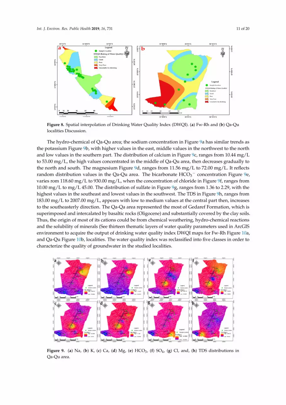
Figure 8. Spatial interpolation of Drinking Water Quality Index (DWQI). (a) Fw-Rh and (b) Qa-Qulocalities Discussion.

The hydro-chemical of Qa-Qu area; the sodium concentration in Figure 9a has similar trends asthe potassium Figure 9b, with higher values in the east, middle values in the northwest to the northand low values in the southern part. The distribution of calcium in Figure 9c, ranges from 10.44 mg/Lto 53.00 mg/L, the high values concentrated in the middle of Qa-Qu area, then decreases gradually tothe north and south. The magnesium Figure 9d, ranges from 11.56 mg/L to 72.00 mg/L. It reflectsrandom distribution values in the Qa-Qu area. The bicarbonate HCO3

− concentration Figure 9e,varies rom 118.60 mg/L to 930.00 mg/L, when the concentration of chloride in Figure 9f, ranges from10.00 mg/L to mg/L 45.00. The distribution of sulfate in Figure 9g, ranges from 1.36 to 2.29, with thehighest values in the southeast and lowest values in the southwest. The TDS in Figure 9h, ranges from183.00 mg/L to 2007.00 mg/L, appears with low to medium values at the central part then, increasesto the southeasterly direction. The Qa-Qa area represented the most of Gedaref Formation, which issuperimposed and intercalated by basaltic rocks (Oligocene) and substantially covered by the clay soils.Thus, the origin of most of its cations could be from chemical weathering, hydro-chemical reactionsand the solubility of minerals (See thirteen thematic layers of water quality parameters used in ArcGISenvironment to acquire the output of drinking water quality index DWQI maps for Fw-Rh Figure 10a,and Qa-Qu Figure 10b, localities. The water quality index was reclassified into five classes in order tocharacterize the quality of groundwater in the studied localities.

Int. J. Environ. Res. Public Health 2019, 16, x FOR PEER REVIEW 11 of 19

random distribution values in the Qa-Qu area. The bicarbonate HCO3− concentration Figure 9e, varies from 118.60 mg/L to 930.00 mg/L, when the concentration of chloride in Figure 9f, ranges from 10.00 mg/L to mg/L 45.00. The distribution of sulfate in Figure 9g, ranges from 1.36 to 2.29, with the highest values in the southeast and lowest values in the southwest. The TDS in Figure 9h, ranges from 183.00 mg/L to 2007.00 mg/L, appears with low to medium values at the central part then, increases to the southeasterly direction. The Qa-Qa area represented the most of Gedaref Formation, which is superimposed and intercalated by basaltic rocks (Oligocene) and substantially covered by the clay soils. Thus, the origin of most of its cations could be from chemical weathering, hydro-chemical reactions and the solubility of minerals (See thirteen thematic layers of water quality parameters used in ArcGIS environment to acquire the output of drinking water quality index DWQI maps for Fw-Rh Figure 10a, and Qa-Qu Figure 10b, localities. The water quality index was reclassified into five classes in order to characterize the quality of groundwater in the studied localities.

Figure 9. (a) Na, (b) K, (c) Ca, (d) Mg, (e) HCO3, (f) SO4, (g) Cl, and, (h) TDS distributions in Qa-Qu area.

Figure 10. Spatial interpolation of Drinking Water Quality Index (DWQI). (a) Fw-Rh and (b) Qa-Qu localities discussion.

3.2. Correlation Matrix

The correlation matrix provides the assessment of the correlation coefficients “r” between groundwater quality elements. These coefficients are applied to suppress the strength of the linear relationship between the variables. It has been used to estimate both positive and negative correlations. The project area describes three examples of groundwater aquifers; (1) sandstone

Figure 9. (a) Na, (b) K, (c) Ca, (d) Mg, (e) HCO3, (f) SO4, (g) Cl, and, (h) TDS distributions inQa-Qu area.

Int. J. Environ. Res. Public Health 2019, 16, 731 12 of 20

Int. J. Environ. Res. Public Health 2019, 16, x FOR PEER REVIEW 11 of 19

random distribution values in the Qa-Qu area. The bicarbonate HCO3− concentration Figure 9e, varies from 118.60 mg/L to 930.00 mg/L, when the concentration of chloride in Figure 9f, ranges from 10.00 mg/L to mg/L 45.00. The distribution of sulfate in Figure 9g, ranges from 1.36 to 2.29, with the highest values in the southeast and lowest values in the southwest. The TDS in Figure 9h, ranges from 183.00 mg/L to 2007.00 mg/L, appears with low to medium values at the central part then, increases to the southeasterly direction. The Qa-Qa area represented the most of Gedaref Formation, which is superimposed and intercalated by basaltic rocks (Oligocene) and substantially covered by the clay soils. Thus, the origin of most of its cations could be from chemical weathering, hydro-chemical reactions and the solubility of minerals (See thirteen thematic layers of water quality parameters used in ArcGIS environment to acquire the output of drinking water quality index DWQI maps for Fw-Rh Figure 10a, and Qa-Qu Figure 10b, localities. The water quality index was reclassified into five classes in order to characterize the quality of groundwater in the studied localities.

Figure 9. (a) Na, (b) K, (c) Ca, (d) Mg, (e) HCO3, (f) SO4, (g) Cl, and, (h) TDS distributions in Qa-Qu area.

Figure 10. Spatial interpolation of Drinking Water Quality Index (DWQI). (a) Fw-Rh and (b) Qa-Qu localities discussion.

3.2. Correlation Matrix

The correlation matrix provides the assessment of the correlation coefficients “r” between groundwater quality elements. These coefficients are applied to suppress the strength of the linear relationship between the variables. It has been used to estimate both positive and negative correlations. The project area describes three examples of groundwater aquifers; (1) sandstone

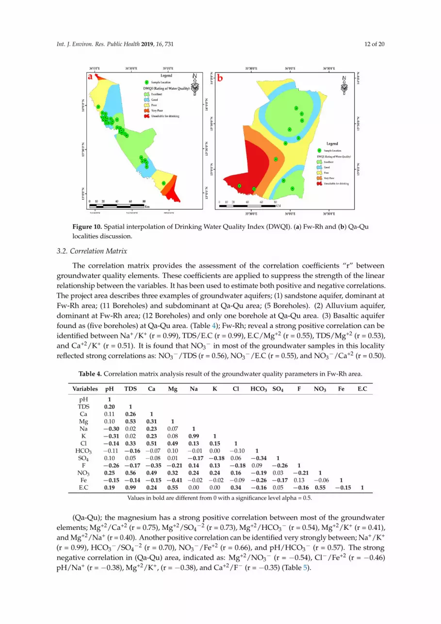
Figure 10. Spatial interpolation of Drinking Water Quality Index (DWQI). (a) Fw-Rh and (b) Qa-Qulocalities discussion.

3.2. Correlation Matrix

The correlation matrix provides the assessment of the correlation coefficients “r” betweengroundwater quality elements. These coefficients are applied to suppress the strength of the linearrelationship between the variables. It has been used to estimate both positive and negative correlations.The project area describes three examples of groundwater aquifers; (1) sandstone aquifer, dominant atFw-Rh area; (11 Boreholes) and subdominant at Qa-Qu area; (5 Boreholes). (2) Alluvium aquifer,dominant at Fw-Rh area; (12 Boreholes) and only one borehole at Qa-Qu area. (3) Basaltic aquiferfound as (five boreholes) at Qa-Qu area. (Table 4); Fw-Rh; reveal a strong positive correlation can beidentified between Na+/K+ (r = 0.99), TDS/E.C (r = 0.99), E.C/Mg+2 (r = 0.55), TDS/Mg+2 (r = 0.53),and Ca+2/K+ (r = 0.51). It is found that NO3

− in most of the groundwater samples in this localityreflected strong correlations as: NO3

−/TDS (r = 0.56), NO3−/E.C (r = 0.55), and NO3

−/Ca+2 (r = 0.50).

Table 4. Correlation matrix analysis result of the groundwater quality parameters in Fw-Rh area.

Variables pH TDS Ca Mg Na K Cl HCO3 SO4 F NO3 Fe E.C

pH 1TDS 0.20 1Ca 0.11 0.26 1Mg 0.10 0.53 0.31 1Na −0.30 0.02 0.23 0.07 1K −0.31 0.02 0.23 0.08 0.99 1Cl −0.14 0.33 0.51 0.49 0.13 0.15 1

HCO3 −0.11 −0.16 −0.07 0.10 −0.01 0.00 −0.10 1SO4 0.10 0.05 −0.08 0.01 −0.17 −0.18 0.06 −0.34 1

F −0.26 −0.17 −0.35 −0.21 0.14 0.13 −0.18 0.09 −0.26 1NO3 0.25 0.56 0.49 0.32 0.24 0.24 0.16 −0.19 0.03 −0.21 1

Fe −0.15 −0.14 −0.15 −0.41 −0.02 −0.02 −0.09 −0.26 −0.17 0.13 −0.06 1E.C 0.19 0.99 0.24 0.55 0.00 0.00 0.34 −0.16 0.05 −0.16 0.55 −0.15 1

Values in bold are different from 0 with a significance level alpha = 0.5.

(Qa-Qu); the magnesium has a strong positive correlation between most of the groundwaterelements; Mg+2/Ca+2 (r = 0.75), Mg+2/SO4

−2 (r = 0.73), Mg+2/HCO3− (r = 0.54), Mg+2/K+ (r = 0.41),

and Mg+2/Na+ (r = 0.40). Another positive correlation can be identified very strongly between; Na+/K+

(r = 0.99), HCO3−/SO4

−2 (r = 0.70), NO3−/Fe+2 (r = 0.66), and pH/HCO3

− (r = 0.57). The strongnegative correlation in (Qa-Qu) area, indicated as: Mg+2/NO3

− (r = −0.54), Cl−/Fe+2 (r = −0.46)pH/Na+ (r = −0.38), Mg+2/K+, (r = −0.38), and Ca+2/F− (r = −0.35) (Table 5).

Int. J. Environ. Res. Public Health 2019, 16, 731 13 of 20

Table 5. Correlation matrix analysis result of the groundwater quality parameters in Qa-Qu area.

Variables pH TDS Ca Mg Na K Cl HCO3 SO4 F NO3 Fe E.C

pH 1TDS 0.09 1Ca 0.15 0.05 1Mg 0.13 −0.09 0.75 1Na −0.38 −0.09 0.04 0.40 1K −0.38 −0.09 0.04 0.41 0.99 1Cl 0.33 0.45 0.29 0.06 −0.19 −0.19 1

HCO3 0.57 −0.21 0.52 0.54 0.00 0.01 −0.07 1SO4 0.24 −0.16 0.37 0.73 0.43 0.44 −0.15 0.70 1

F −0.27 −0.22 −0.35 −0.18 −0.09 −0.09 −0.16 −0.42 −0.30 1NO3 −0.26 0.06 −0.19 −0.54 −0.15 −0.15 −0.34 −0.08 −0.50 −0.16 1

Fe 0.18 −0.16 −0.05 −0.26 −0.29 −0.29 −0.46 0.08 −0.27 −0.11 0.66 1E.C −0.13 0.24 −0.16 −0.04 0.14 0.16 0.13 0.17 0.34 −0.27 0.15 −0.23 1

Values in bold are different from 0 with a significance level alpha = 0.5.

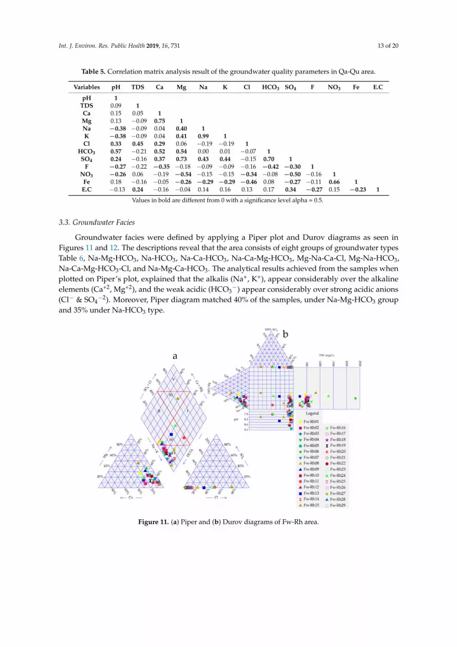
3.3. Groundwater Facies

Groundwater facies were defined by applying a Piper plot and Durov diagrams as seen inFigures 11 and 12. The descriptions reveal that the area consists of eight groups of groundwater typesTable 6, Na-Mg-HCO3, Na-HCO3, Na-Ca-HCO3, Na-Ca-Mg-HCO3, Mg-Na-Ca-Cl, Mg-Na-HCO3,Na-Ca-Mg-HCO3-Cl, and Na-Mg-Ca-HCO3. The analytical results achieved from the samples whenplotted on Piper’s plot, explained that the alkalis (Na+, K+), appear considerably over the alkalineelements (Ca+2, Mg+2), and the weak acidic (HCO3

−) appear considerably over strong acidic anions(Cl− & SO4

−2). Moreover, Piper diagram matched 40% of the samples, under Na-Mg-HCO3 groupand 35% under Na-HCO3 type.

Int. J. Environ. Res. Public Health 2019, 16, x FOR PEER REVIEW 13 of 19

& SO4−2). Moreover, Piper diagram matched 40% of the samples, under Na-Mg-HCO3 group and 35% under Na-HCO3 type.

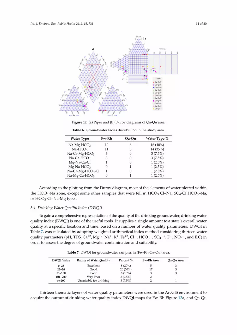
According to the plotting from the Durov diagram, most of the elements of water plotted within the HCO3·Na zone, except some other samples that were fell in HCO3 Cl–Na, SO4·Cl·HCO3–Na, or HCO3·Cl–Na·Mg types.

Figure 11. (a) Piper and (b) Durov diagrams of Fw-Rh area.

Table 6. Groundwater facies distribution in the study area.

Water Type Fw-Rh Qa-Qu Water Type % Na-Mg-HCO3 10 6 16 (40%)

Na-HCO3 11 3 14 (35%) Na-Ca-Mg-HCO3 3 0 3 (7.5%)

Na-Ca-HCO3 3 0 3 (7.5%) Mg-Na-Ca-Cl 1 0 1 (2.5%) Mg-Na-HCO3 0 1 1 (2.5%)

Na-Ca-Mg-HCO3-Cl 1 0 1 (2.5%) Na-Mg-Ca-HCO3 0 1 1 (2.5%)

Figure 12. (a) Piper and (b) Durov diagrams of Qa-Qu area.

Figure 11. (a) Piper and (b) Durov diagrams of Fw-Rh area.

Int. J. Environ. Res. Public Health 2019, 16, 731 14 of 20

Int. J. Environ. Res. Public Health 2019, 16, x FOR PEER REVIEW 13 of 19

& SO4−2). Moreover, Piper diagram matched 40% of the samples, under Na-Mg-HCO3 group and 35% under Na-HCO3 type.

According to the plotting from the Durov diagram, most of the elements of water plotted within the HCO3·Na zone, except some other samples that were fell in HCO3 Cl–Na, SO4·Cl·HCO3–Na, or HCO3·Cl–Na·Mg types.

Figure 11. (a) Piper and (b) Durov diagrams of Fw-Rh area.

Table 6. Groundwater facies distribution in the study area.

Water Type Fw-Rh Qa-Qu Water Type % Na-Mg-HCO3 10 6 16 (40%)

Na-HCO3 11 3 14 (35%) Na-Ca-Mg-HCO3 3 0 3 (7.5%)

Na-Ca-HCO3 3 0 3 (7.5%) Mg-Na-Ca-Cl 1 0 1 (2.5%) Mg-Na-HCO3 0 1 1 (2.5%)

Na-Ca-Mg-HCO3-Cl 1 0 1 (2.5%) Na-Mg-Ca-HCO3 0 1 1 (2.5%)

Figure 12. (a) Piper and (b) Durov diagrams of Qa-Qu area. Figure 12. (a) Piper and (b) Durov diagrams of Qa-Qu area.

Table 6. Groundwater facies distribution in the study area.

Water Type Fw-Rh Qa-Qu Water Type %

Na-Mg-HCO3 10 6 16 (40%)Na-HCO3 11 3 14 (35%)

Na-Ca-Mg-HCO3 3 0 3 (7.5%)Na-Ca-HCO3 3 0 3 (7.5%)Mg-Na-Ca-Cl 1 0 1 (2.5%)Mg-Na-HCO3 0 1 1 (2.5%)

Na-Ca-Mg-HCO3-Cl 1 0 1 (2.5%)Na-Mg-Ca-HCO3 0 1 1 (2.5%)

According to the plotting from the Durov diagram, most of the elements of water plotted withinthe HCO3·Na zone, except some other samples that were fell in HCO3 Cl–Na, SO4·Cl·HCO3–Na,or HCO3·Cl–Na·Mg types.

3.4. Drinking Water Quality Index (DWQI)

To gain a comprehensive representation of the quality of the drinking groundwater, drinking waterquality index (DWQI) is one of the useful tools. It supplies a single amount to a state’s overall waterquality at a specific location and time, based on a number of water quality parameters. DWQI inTable 7, was calculated by adopting weighted arithmetical index method considering thirteen waterquality parameters (pH, TDS, Ca+2, Mg+2, Na+, K+, Fe+2, Cl−, HCO3

−, SO4−2, F−, NO3

−, and E.C) inorder to assess the degree of groundwater contamination and suitability.

Table 7. DWQI for groundwater samples in (Fw-Rh-Qa-Qu) area.

DWQI Value Rating of Water Quality Percent % Fw-Rh Area Qa-Qu Area

0–25 Excellent 8 (20%) 5 325–50 Good 20 (50%) 17 3

51–100 Poor 6 (15%) 3 3101–200 Very Poor 3 (7.5%) 2 1>>200 Unsuitable for drinking 3 (7.5%) 2 1

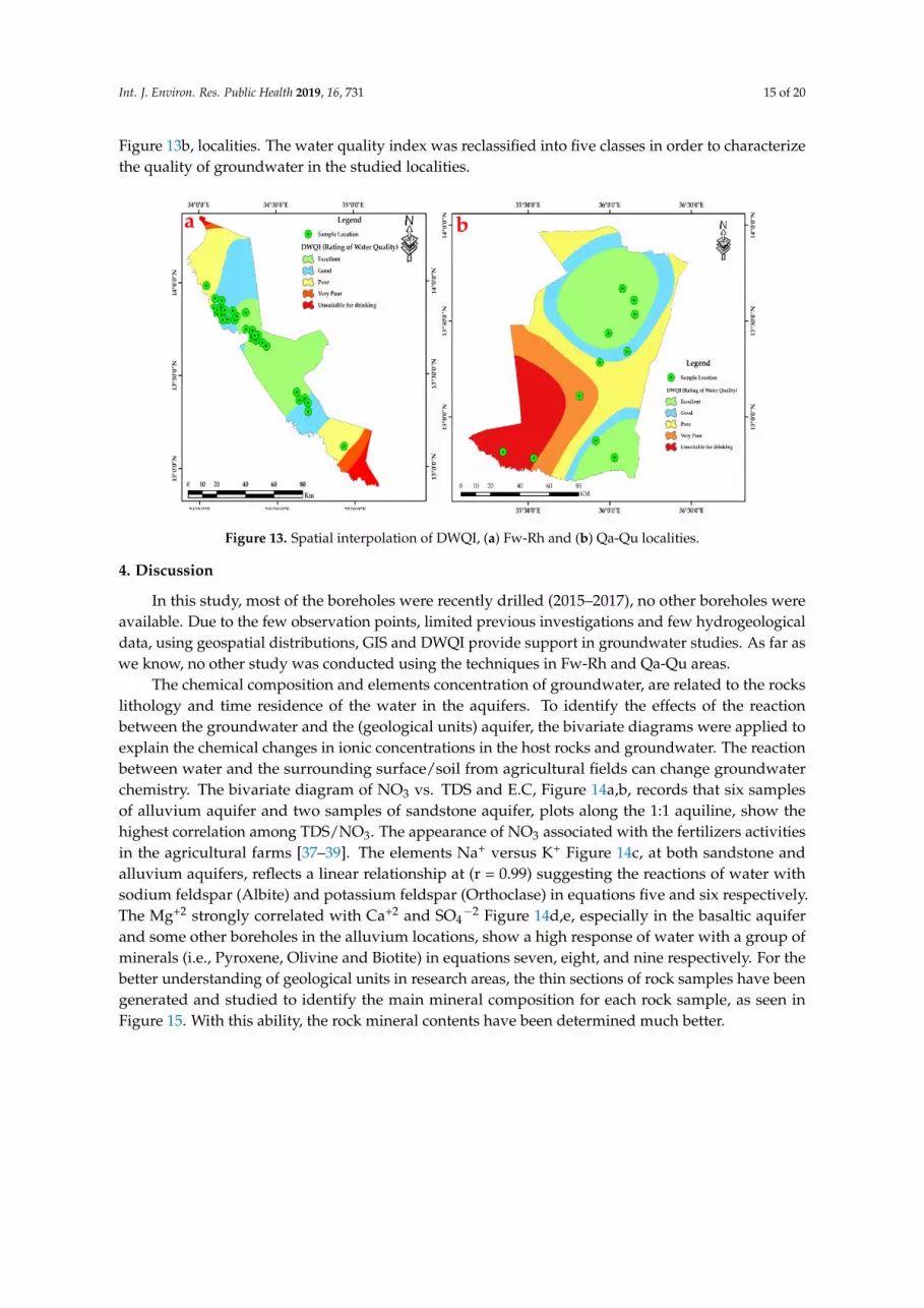
Thirteen thematic layers of water quality parameters were used in the ArcGIS environment toacquire the output of drinking water quality index DWQI maps for Fw-Rh Figure 13a, and Qa-Qu

Int. J. Environ. Res. Public Health 2019, 16, 731 15 of 20

Figure 13b, localities. The water quality index was reclassified into five classes in order to characterizethe quality of groundwater in the studied localities.

Int. J. Environ. Res. Public Health 2019, 16, x FOR PEER REVIEW 14 of 19

3.4. Drinking Water Quality Index (DWQI)

To gain a comprehensive representation of the quality of the drinking groundwater, drinking water quality index (DWQI) is one of the useful tools. It supplies a single amount to a state’s overall water quality at a specific location and time, based on a number of water quality parameters. DWQI in Table 7, was calculated by adopting weighted arithmetical index method considering thirteen water quality parameters (pH, TDS, Ca+2, Mg+2, Na+, K+, Fe+2, Cl−, HCO3−, SO4−2, F−, NO3−, and E.C) in order to assess the degree of groundwater contamination and suitability.

Table 7. DWQI for groundwater samples in (Fw-Rh-Qa-Qu) area.

DWQI Value Rating of Water Quality Percent % Fw-Rh Area Qa-Qu Area 0–25 Excellent 8 (20%) 5 3

25–50 Good 20 (50%) 17 3 51–100 Poor 6 (15%) 3 3

101–200 Very Poor 3 (7.5%) 2 1 >>200 Unsuitable for drinking 3 (7.5%) 2 1

Thirteen thematic layers of water quality parameters were used in the ArcGIS environment to acquire the output of drinking water quality index DWQI maps for Fw-Rh Figure 13a, and Qa-Qu Figure 13b, localities. The water quality index was reclassified into five classes in order to characterize the quality of groundwater in the studied localities.

Figure 13. Spatial interpolation of DWQI, (a) Fw-Rh and (b) Qa-Qu localities.

4. Discussion

In this study, most of the boreholes were recently drilled (2015–2017), no other boreholes were available. Due to the few observation points, limited previous investigations and few hydrogeological data, using geospatial distributions, GIS and DWQI provide support in groundwater studies. As far as we know, no other study was conducted using the techniques in Fw-Rh and Qa-Qu areas.

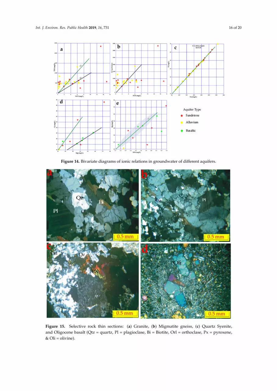
The chemical composition and elements concentration of groundwater, are related to the rocks lithology and time residence of the water in the aquifers. To identify the effects of the reaction between the groundwater and the (geological units) aquifer, the bivariate diagrams were applied to explain the chemical changes in ionic concentrations in the host rocks and groundwater. The reaction between water and the surrounding surface/soil from agricultural fields can change groundwater chemistry. The bivariate diagram of NO3 vs. TDS and E.C, Figure 14a,b, records that six samples of alluvium aquifer and two samples of sandstone aquifer, plots along the 1:1 aquiline, show the highest

Figure 13. Spatial interpolation of DWQI, (a) Fw-Rh and (b) Qa-Qu localities.

4. Discussion

In this study, most of the boreholes were recently drilled (2015–2017), no other boreholes wereavailable. Due to the few observation points, limited previous investigations and few hydrogeologicaldata, using geospatial distributions, GIS and DWQI provide support in groundwater studies. As far aswe know, no other study was conducted using the techniques in Fw-Rh and Qa-Qu areas.

The chemical composition and elements concentration of groundwater, are related to the rockslithology and time residence of the water in the aquifers. To identify the effects of the reactionbetween the groundwater and the (geological units) aquifer, the bivariate diagrams were applied toexplain the chemical changes in ionic concentrations in the host rocks and groundwater. The reactionbetween water and the surrounding surface/soil from agricultural fields can change groundwaterchemistry. The bivariate diagram of NO3 vs. TDS and E.C, Figure 14a,b, records that six samplesof alluvium aquifer and two samples of sandstone aquifer, plots along the 1:1 aquiline, show thehighest correlation among TDS/NO3. The appearance of NO3 associated with the fertilizers activitiesin the agricultural farms [37–39]. The elements Na+ versus K+ Figure 14c, at both sandstone andalluvium aquifers, reflects a linear relationship at (r = 0.99) suggesting the reactions of water withsodium feldspar (Albite) and potassium feldspar (Orthoclase) in equations five and six respectively.The Mg+2 strongly correlated with Ca+2 and SO4

−2 Figure 14d,e, especially in the basaltic aquiferand some other boreholes in the alluvium locations, show a high response of water with a group ofminerals (i.e., Pyroxene, Olivine and Biotite) in equations seven, eight, and nine respectively. For thebetter understanding of geological units in research areas, the thin sections of rock samples have beengenerated and studied to identify the main mineral composition for each rock sample, as seen inFigure 15. With this ability, the rock mineral contents have been determined much better.

Int. J. Environ. Res. Public Health 2019, 16, 731 16 of 20

Int. J. Environ. Res. Public Health 2019, 16, x FOR PEER REVIEW 15 of 19

correlation among TDS/NO3. The appearance of NO3 associated with the fertilizers activities in the agricultural farms [38–40]. The elements Na+ versus K+ Figure 14c, at both sandstone and alluvium aquifers, reflects a linear relationship at (r = 0.99) suggesting the reactions of water with sodium feldspar (Albite) and potassium feldspar (Orthoclase) in equations five and six respectively. The Mg+2 strongly correlated with Ca+2 and SO4−2 Figure 14d,e, especially in the basaltic aquifer and some other boreholes in the alluvium locations, show a high response of water with a group of minerals (i.e., Pyroxene, Olivine and Biotite) in equations seven, eight, and nine respectively. For the better understanding of geological units in research areas, the thin sections of rock samples have been generated and studied to identify the main mineral composition for each rock sample, as seen in Figure 15. With this ability, the rock mineral contents have been determined much better.

The main mechanism for the dissolution of rock minerals that releases the element such as: (Ca, Mg, Na, K and HCO3); into the groundwater, have been indicated in the following reactions: (Pl)Anorthite: CaAl Si O + 2CO + H O → Al Si O (OH) + Ca + 2HCO (4) (Pl)Albite: 2NaAl O + 9H O + 2H → Al Si O (OH) + 4H SiO + 2Na (5) (Orl) Orthoclase: 2KAlSi O + 11H O → Si O Al (OH) + 2K + 2OH (6) (Px)Pyroxene: CaMg(Si O ) + 4CO + 6H O → Ca + Mg 4HCO + 2Si(OH) (7) (Oli)Olivine(Fe, Mg )SiO + 4H CO → 2(Fe, Mg ) + H SiO + 4HCO (8) (Bi) Biotite: K(Mg, Fe) (AlSi O )(F, OH ) + 5H O + 4CO ) → K + Mg + Fe(OH) + 4HCO + H + 2F

(9)

Figure 14. Bivariate diagrams of ionic relations in groundwater of different aquifers. Figure 14. Bivariate diagrams of ionic relations in groundwater of different aquifers.Int. J. Environ. Res. Public Health 2019, 16, x FOR PEER REVIEW 16 of 19

Figure 15. Selective rock thin sections: (a) Granite, (b) Migmatite gneiss, (c) Quartz Syenite, and Oligocene basalt (Qtz = quartz, Pl = plagioclase, Bi = Biotite, Orl = orthoclase, Px = pyroxene, & Oli = olivine).

5. Conclusions

This study explains the geospatial distribution, adopting statistical methods with GIS to characteristics and mapped the groundwater quality in the different hydrogeological units such as sandstone, alluvium, and basaltic aquifers, which are located in eastern Sudan (the southwestern part of Gedaref State). Forty water boreholes samples from different locations were collected, analyzed and estimated.

Aqua Chem v.2014.2 software has been used for groundwater quality elements analysis, while ArcGIS software was chosen for the interpretation and spatial mapping, so that groundwater quality estimation studies have been completed successfully. This study envisions the significance of graphical illustrations, i.e., Piper, Bivariate, Dendrogram, and Durov diagrams plot, to determine variation in hydro-chemical facies and to understand the evolution of hydro-chemical processes in Qa-Qu and Fw-Rh areas.

The hydrogeochemical evaluation outcomes and distribution of groundwater cations (Na+, Ca+2, K+, Mg+2) and anions (HCO3−, Cl−, SO4−2, F−) in both the Qa-Qu and Fw-Rh areas, shows that the groundwater is chemically affected by aquifer lithology. According to the plotting from the Durov diagram, most of the elements of water plotted within the HCO3·Na zone, except some other samples that fell in HCO3 Cl–Na, SO4·Cl·HCO3–Na, or HCO3·Cl–Na Mg types. With the exclusion of a few elements, the quality of groundwater is mostly suitable for drinking purposes and other domestic uses. The groundwater in this project is controlled by sodium and bicarbonate ions, which define the composition of the water type to be Na HCO3. According to this investigation, three potential aquifers (sandstone, alluvium, and basalt); have been identified in the research areas.

The DWQI was used to determine the groundwater quality and its suitability for drinking purposes. According to this investigation, 20% of groundwater samples represent ‘‘excellent water’’, 50% indicate ‘‘good water’’, 15% represent ‘‘poor water’’, 7.5% shows ‘‘very poor water’’, and 7.5%

Figure 15. Selective rock thin sections: (a) Granite, (b) Migmatite gneiss, (c) Quartz Syenite,and Oligocene basalt (Qtz = quartz, Pl = plagioclase, Bi = Biotite, Orl = orthoclase, Px = pyroxene,& Oli = olivine).

Int. J. Environ. Res. Public Health 2019, 16, 731 17 of 20

The main mechanism for the dissolution of rock minerals that releases the element such as:(Ca, Mg, Na, K and HCO3); into the groundwater, have been indicated in the following reactions:

(Pl)Anorthite : CaAl2Si2O3 + 2CO3 + H2O → Al2Si2O5(OH)4 + Ca+2 + 2HCO3 (4)

(Pl)Albite : 2NaAl3O8 + 9H2O + 2H+ → Al2Si2O5(OH)4 + 4H4SiO4 + 2Na+ (5)

(Orl) Orthoclase : 2KAlSi3O8 + 11H2O → Si2O5Al2(OH)4 + 2K+ + 2OH− (6)

(Px)Pyroxene : CaMg(Si2O6) + 4CO2 + 6H2O → Ca2+ + Mg2+ 4HCO−3 + 2Si(OH)4 (7)

(Oli)Olivine(

Fe, Mg2+)

SiO4 + 4H2CO3 → 2(

Fe, Mg2+)+ H4SiO4 + 4HCO−3 (8)

(Bi) Biotite : K(Mg, Fe)3(AlSi3O10)(F, OH2) + 5H2O + 4CO2) → K + Mg + Fe(OH)3 + 4HCO3 + H + 2F (9)

5. Conclusions

This study explains the geospatial distribution, adopting statistical methods with GIS tocharacteristics and mapped the groundwater quality in the different hydrogeological units suchas sandstone, alluvium, and basaltic aquifers, which are located in eastern Sudan (the southwesternpart of Gedaref State). Forty water boreholes samples from different locations were collected,analyzed and estimated.

Aqua Chem v.2014.2 software has been used for groundwater quality elements analysis,while ArcGIS software was chosen for the interpretation and spatial mapping, so that groundwaterquality estimation studies have been completed successfully. This study envisions the significanceof graphical illustrations, i.e., Piper, Bivariate, Dendrogram, and Durov diagrams plot, to determinevariation in hydro-chemical facies and to understand the evolution of hydro-chemical processes inQa-Qu and Fw-Rh areas.

The hydrogeochemical evaluation outcomes and distribution of groundwater cations (Na+, Ca+2,K+, Mg+2) and anions (HCO3

−, Cl−, SO4−2, F−) in both the Qa-Qu and Fw-Rh areas, shows that the

groundwater is chemically affected by aquifer lithology. According to the plotting from the Durovdiagram, most of the elements of water plotted within the HCO3·Na zone, except some other samplesthat fell in HCO3 Cl–Na, SO4·Cl·HCO3–Na, or HCO3·Cl–Na Mg types. With the exclusion of a fewelements, the quality of groundwater is mostly suitable for drinking purposes and other domesticuses. The groundwater in this project is controlled by sodium and bicarbonate ions, which define thecomposition of the water type to be Na HCO3. According to this investigation, three potential aquifers(sandstone, alluvium, and basalt); have been identified in the research areas.

The DWQI was used to determine the groundwater quality and its suitability for drinkingpurposes. According to this investigation, 20% of groundwater samples represent “excellent water”,50% indicate “good water”, 15% represent “poor water”, 7.5% shows “very poor water”, and 7.5%appear as “unsuitable for drinking”. The drinking water quality index that was produced for this studyreveals that the northwest and southeast parts of Fw-Rh and the southwest part of Qa-Qu locationshas the poorest water quality, which is classified as “unsuitable for drinking”.

It should be noted, that the actual variations in spatial interpolations, can considerably divergefrom the values predicted by spatial interpolation, it may lead to probable limitations of Krigingespecially when data is scarce and unequally distributed. Thus, it is essential to know the number ofdata locations and the geographical extent of the region containing those data locations. In this case,one of the crucial steps is estimating the variogram model, which is more difficult with a small numberof data locations. In this study, the transformations (Log & BoxCox), have been used to make thedata normally distributed and satisfy the assumption of equal variability for the data. Several typesof semivariogram models were tested in Table 3, for all water quality parameters to achieve morereliable results.

Int. J. Environ. Res. Public Health 2019, 16, 731 18 of 20

Author Contributions: T.H., B.A.E. & J.Z. had the initial idea for the research project and writing of the article,M.M.B., W.A. & B.A.E. accomplished fieldwork, data acquisition and implemented the research experiments,K.M.E. & E.H.A. helping in data analysis and maps layout, H.T. supervise the plan and evaluate the conclusion ofthe manuscript.

Funding: This study financially supported by the Sichuan Environmental Engineering Assessment Center ProjectTechnical Consultation on Comprehensive Assessment of Groundwater Pollution Status in Typical Industrial Parkof Shiyang, Deyang (2017H01013).

Acknowledgments: The authors thank the Water Corporation of Gedaref State—Sudan (WCGSS) and WaterEnvironmental Sanitation (WES), Project Gedaref State—Sudan; for the technical support of this study.

Conflicts of Interest: The authors declare no conflict of interest.

References

1. Li, P.; Wu, J.; Tian, R.; He, S.; He, X.; Xue, C.; Zhang, K. Geochemistry, hydraulic connectivity and qualityappraisal of multilayered groundwater in the Hongdunzi coal mine, northwest China. Mine Water Environ.2018, 37, 222–237. [CrossRef]

2. Ferchichi, H.; Hamouda, M.B.; Farhat, B.; Mammou, A.B. Assessment of groundwater salinity using GIS andmultivariate statistics in a coastal Mediterranean aquifer. Int. J. Environ. Sci. Technol. 2018, 15, 2473–2492.[CrossRef]

3. Tiwari, A.K.; Ghione, R.; De Maio, M.; Lavy, M. Evaluation of hydrogeochemical processes and groundwaterquality for suitability of drinking and irrigation purposes: A case study in the Aosta Valley region, Italy.Arabian J. Geosci. 2017, 10, 264. [CrossRef]

4. Kura, N.U.; Ramli, M.F.; Sulaiman, W.N.A.; Ibrahim, S.; Aris, A.Z.; Mustapha, A. Evaluation of factorsinfluencing the groundwater chemistry in a small tropical island of Malaysia. Int. J. Environ. Res. Public Health2013, 10, 1861–1881. [CrossRef] [PubMed]

5. Bhusari, V.; Katpatal, Y.; Kundal, P. Performance evaluation of a reverse-gradient artificial recharge systemin basalt aquifers of Maharashtra, India. Hydrogeol. J. 2017, 25, 689–706. [CrossRef]

6. Vesali Naseh, M.R.; Noori, R.; Berndtsson, R.; Adamowski, J.; Sadatipour, E. Groundwater Pollution SourcesApportionment in the Ghaen Plain, Iran. Int. J. Environ. Res. Public Health 2018, 15, 172. [CrossRef] [PubMed]

7. Appelo, C.A.J.; Postma, D. Geochemistry, Groundwater and Pollution; CRC Press: Amsterdam, The Netherlands,2004; p. 647.

8. Chacha, N.; Njau, K.N.; Lugomela, G.V.; Muzuka, A.N. Hydrogeochemical characteristics and spatialdistribution of groundwater quality in Arusha well fields, Northern Tanzania. Appl. Water Sci. 2018, 8, 118.[CrossRef]

9. Nelly, K.C.; Mutua, F. Ground Water Quality Assessment Using GIS and Remote Sensing: A Case Study ofJuja Location, Kenya. Am. J. Geogr. Inf. Syst. 2016, 5, 12–23.

10. Ravikumar, P.; Somashekar, R. Principal component analysis and hydrochemical facies characterization toevaluate groundwater quality in Varahi river basin, Karnataka state, India. Appl. Water Sci. 2017, 7, 745–755.[CrossRef]

11. Varol, S.; Davraz, A. Evaluation of the groundwater quality with WQI (Water Quality Index) and multivariateanalysis: A case study of the Tefenni plain (Burdur/Turkey). Environ. Earth Sci. 2015, 73, 1725–1744.[CrossRef]

12. Eang, K.E.; Igarashi, T.; Kondo, M.; Nakatani, T.; Tabelin, C.B.; Fujinaga, R. Groundwater monitoring ofan open-pit limestone quarry: Water-rock interaction and mixing estimation within the rock layers bygeochemical and statistical analyses. Int. J. Min. Sci. Technol. 2018, 28, 849–857. [CrossRef]

13. Ahmed, A.; Clark, I. Groundwater flow and geochemical evolution in the Central Flinders Ranges,South Australia. Sci. Total Environ. 2016, 572, 837–851. [CrossRef] [PubMed]

14. Tóth, J. Groundwater as a geologic agent: An overview of the causes, processes, and manifestations.Hydrogeol. J. 1999, 7, 1–14. [CrossRef]

15. Zaki, S.R.; Redwan, M.; Masoud, A.M.; Moneim, A.A.A. Chemical characteristics and assessment of groundwaterquality in Halayieb area, southeastern part of the Eastern Desert, Egypt. Geosci. J. 2018, 23, 149–164. [CrossRef]

16. Gidey, A. Geospatial distribution modeling and determining suitability of groundwater quality for irrigationpurpose using geospatial methods and water quality index (WQI) in Northern Ethiopia. Appl. Water Sci.2018, 8, 82. [CrossRef]

Int. J. Environ. Res. Public Health 2019, 16, 731 19 of 20

17. Lawrence, A.; Gooddy, D.; Kanatharana, P.; Meesilp, W.; Ramnarong, V. Groundwater evolution beneathHat Yai, a rapidly developing city in Thailand. Hydrogeol. J. 2000, 8, 564–575.

18. Edmunds, W.; Ma, J.; Aeschbach-Hertig, W.; Kipfer, R.; Darbyshire, D. Groundwater recharge history andhydrogeochemical evolution in the Minqin Basin, North West China. Appl. Geochem. 2006, 21, 2148–2170.[CrossRef]

19. Castilla-Hernández, P.; del Rocío Torres-Alvarado, M.; Herrera-San Luis, J.A.; Cruz-López, N. Water quality ofa reservoir and its major tributary located in east-central Mexico. Int. J. Environ. Res. Public Health 2014, 11, 6119–6135.[CrossRef] [PubMed]

20. Pande, C.B.; Moharir, K. Spatial analysis of groundwater quality mapping in hard rock area in the Akola andBuldhana districts of Maharashtra, India. Appl. Water Sci. 2018, 8, 106. [CrossRef]

21. Das, S.; Behera, S.; Kar, A.; Narendra, P.; Guha, S. Hydrogeomorphological mapping in ground waterexploration using remotely sensed data—A case study in keonjhar district, orissa. J. Indian Soc. Remote Sens.1997, 25, 247–259. [CrossRef]

22. Abdalla, F. Mapping of groundwater prospective zones using remote sensing and GIS techniques: A casestudy from the Central Eastern Desert, Egypt. J. Afr. Earth Sci. 2012, 70, 8–17. [CrossRef]

23. Moubark, K.; Abdelkareem, M. Characterization and assessment of groundwater resources using hydrogeochemicalanalysis, GIS, and field data in southern Wadi Qena, Egypt. Arabian J. Geosci. 2018, 11, 598. [CrossRef]

24. Sener, S.; Sener, E.; Davraz, A. Evaluation of water quality using water quality index (WQI) method and GISin Aksu River (SW-Turkey). Sci. Total Environ. 2017, 584, 131–144. [CrossRef] [PubMed]

25. Sahu, P.; Sikdar, P.J.E.G. Hydrochemical framework of the aquifer in and around East Kolkata Wetlands,West Bengal, India. Environ. Geol. 2008, 55, 823–835. [CrossRef]

26. Rubio-Arias, H.; Contreras-Caraveo, M.; Quintana, R.M.; Saucedo-Teran, R.A.; Pinales-Munguia, A.An overall water quality index (WQI) for a man-made aquatic reservoir in Mexico. Int. J. Environ. Res.Public Health 2012, 9, 1687–1698. [CrossRef] [PubMed]

27. De La Mora-Orozco, C.; Flores-Lopez, H.; Rubio-Arias, H.; Chavez-Duran, A.; Ochoa-Rivero, J.Developing a water quality index (WQI) for an irrigation dam. Int. J. Environ. Res. Public Health 2017, 14, 439.[CrossRef] [PubMed]

28. Iqbal, M.; Shoaib, M.; Farid, H.; Lee, J. Assessment of Water Quality Profile Using Numerical ModelingApproach in Major Climate Classes of Asia. Int. J. Environ. Res. Public Health 2018, 15, 2258. [CrossRef][PubMed]

29. Ravikumar, P.; Somashekar, R.; Prakash, K. A comparative study on usage of Durov and Piper diagrams tointerpret hydrochemical processes in groundwater from SRLIS river basin, Karnataka, India. Elixir Earth Sci.2015, 80, 31073–31077.

30. Wu, Z.; Wang, X.; Chen, Y.; Cai, Y.; Deng, J. Assessing river water quality using water quality index in LakeTaihu Basin, China. Sci. Total Environ. 2018, 612, 914–922. [CrossRef] [PubMed]

31. Misaghi, F.; Delgosha, F.; Razzaghmanesh, M.; Myers, B. Introducing a water quality index for assessingwater for irrigation purposes: A case study of the Ghezel Ozan River. Sci. Total Environ. 2017, 589, 107–116.[CrossRef] [PubMed]

32. Tameim, O.; Zakaria, Z.; Hussein, H.; el Gaddal, A.A.; Jobin, W.R. Control of schistosomiasis in the newRahad Irrigation Scheme of Central Sudan. J. Trop. Med. Hyg. 1985, 88, 115–124. [PubMed]

33. World Health Organization. Guidelines for drinking-water quality: First addendum to the fourth edition;World Health Organization: Geneva, Switzerland, 2017; p. 631.

34. Ibrahim, K.; Hussein, M.; Giddo, I. Application of combined geophysical and hydrogeological techniquesto groundwater exploration: A case study of Showak-Wad Elhelew area, Eastern Sudan. J. Afr. Earth Sci.1992, 15, 1–10. [CrossRef]

35. Eisawi, A.; Schrank, E. Terrestrial palynology and age assessment of the Gedaref Formation (eastern Sudan).J. Afr. Earth Sci. 2009, 54, 22–30. [CrossRef]

36. Wipki, M.; Germann, K.; Schwarz, T. Alunitic kaolins of the Gedaref region (NE-Sudan). In GeoscientificResearch in Northeast Africa; CRC Press: Berlin, Germany, 2017; pp. 509–514.

37. Dawelbeit, M.I.; Babiker, E.J.S. Effect of tillage and method of sowing on wheat yield in irrigated Vertisols ofRahad, Sudan. Soil Tillage Res. 1997, 42, 127–132. [CrossRef]

Int. J. Environ. Res. Public Health 2019, 16, 731 20 of 20

38. Saunders, D.A. Wheat in Heat-stressed Environments: Irrigated, Dry Areas, and Rice-wheat Farming Systems:Proceedings of the International Conferences: Wheat in Hot, Dry, Irrigated Environments, Wad Medani, Sudan,1-4 February 1993, Wheat in Warm Area, Rice-wheat Farming Systems, Dinajpur, Bangladesh, 13-15 Feburary [sic]1993; CIMMYT: Wad Medani, Sudan, 1994; p. 415.

39. Mozafar, A. Nitrogen fertilizers and the amount of vitamins in plants: A review. J. Plant Nutr. 1993, 16, 2479–2506.[CrossRef]

© 2019 by the authors. Licensee MDPI, Basel, Switzerland. This article is an open accessarticle distributed under the terms and conditions of the Creative Commons Attribution(CC BY) license (http://creativecommons.org/licenses/by/4.0/).