Multiple scattering and accidental coincidences in the J-PET detector simulated using GATE package P. Kowalski a , P. Moskal b , W. Wi´ slicki a , L. Raczy´ nski a , T. Bednarski b , P. Bia las b , J. Bu lka c , E. Czerwi´ nski b , A. Gajos b , A. Gruntowski b , D. Kami´ nska b , L. Kap lon b,d , A. Kochanowski e , G. Korcyl b , J. Kowal b , T. Kozik b , W. Krzemie´ n f , E. Kubicz b , Sz. Nied´ zwiecki b , M. Pa lka b , Z. Rudy b , P. Salabura b , N.G. Sharma b , M. Silarski b , A. S lomski b , J. Smyrski b , A. Strzelecki b , A. Wieczorek b,d , I. Wochlik c , M. Zieli´ nski b , N. Zo´ n b a ´ Swierk Computing Centre, National Centre for Nuclear Research, 05-400 Otwock- ´ Swierk, Poland b Faculty of Physics, Astronomy and Applied Computer Science, Jagiellonian University, 30-348 Cracow, Poland c Department of Automatics and Bioengineering, AGH University of Science and Technology, Cracow, Poland d Institute of Metallurgy and Materials Science of Polish Academy of Sciences, 30-059 Cracow, Poland e Faculty of Chemistry, Jagiellonian University, 30-060 Cracow, Poland f High Energy Physics Division, National Centre for Nuclear Research, 05-400 Otwock- ´ Swierk, Poland February 17, 2015 PACS: 29.40.Mc, 87.57.uk, 87.10.Rt, 34.50.-s Abstract Novel Positron Emission Tomography system, based on plastic scin- tillators, is developed by the J-PET collaboration. In order to optimize geometrical configuration of built device, advanced computer simulations are performed. Detailed study is presented of background given by acci- dental coincidences and multiple scattering of gamma quanta. 1 Introduction The GEANT4 Application for Tomographic Emission (GATE [1]) represents one of the most advanced specialized software packages for simulations of PET 1 arXiv:1502.04532v1 [physics.ins-det] 16 Feb 2015
Transcript
Multiple scattering and accidental coincidences
in the J-PET detector
simulated using GATE package
P. Kowalskia, P. Moskalb, W. Wislickia, L. Raczynskia,T. Bednarskib, P. Bia lasb, J. Bu lkac, E. Czerwinskib, A. Gajosb,A. Gruntowskib, D. Kaminskab, L. Kap lonb,d, A. Kochanowskie,G. Korcylb, J. Kowalb, T. Kozikb, W. Krzemienf , E. Kubiczb,
Sz. Niedzwieckib, M. Pa lkab, Z. Rudyb, P. Salaburab,N.G. Sharmab, M. Silarskib, A. S lomskib, J. Smyrskib,
A. Strzeleckib, A. Wieczorekb,d, I. Wochlikc, M. Zielinskib, N. Zonb
aSwierk Computing Centre, National Centre for Nuclear Research,05-400 Otwock-Swierk, Poland
bFaculty of Physics, Astronomy and Applied Computer Science,Jagiellonian University, 30-348 Cracow, Poland
cDepartment of Automatics and Bioengineering, AGH Universityof Science and Technology, Cracow, Poland
dInstitute of Metallurgy and Materials Science of Polish Academyof Sciences, 30-059 Cracow, Poland
eFaculty of Chemistry, Jagiellonian University, 30-060 Cracow,Poland
fHigh Energy Physics Division, National Centre for NuclearResearch, 05-400 Otwock-Swierk, Poland
February 17, 2015
PACS: 29.40.Mc, 87.57.uk, 87.10.Rt, 34.50.-s
Abstract
Novel Positron Emission Tomography system, based on plastic scin-tillators, is developed by the J-PET collaboration. In order to optimizegeometrical configuration of built device, advanced computer simulationsare performed. Detailed study is presented of background given by acci-dental coincidences and multiple scattering of gamma quanta.
1 Introduction
The GEANT4 Application for Tomographic Emission (GATE [1]) representsone of the most advanced specialized software packages for simulations of PET
1
arX
iv:1
502.
0453
2v1
[ph
ysic
s.in
s-de
t] 1
6 Fe
b 20
15
scanners. Despite the complexity of the simulated system, GATE is easily con-figurable and facilitates convenient use of the powerful GEANT4 simulationtoolkit.
Thanks to the fact, that the software was widely verified, it may be usedfor simulations of such a prototype devices as Strip-PET scanner [2]-[4], buildby the J-PET collaboration. The scanner is based on the plastic scintillatorsrepresenting innovative approach in the field of PET tomography. Another im-portant feature of the scanner is large axial field-of-view (AFOV). PET scannerswith large AFOV are also developed by other collaborations [5]-[14].
2 Setting parameteres of the simulations in theGATE software
Properties of the scintillating material and the detecting surface, were set usingthree GATE-specific files: GateMaterials.db, Materials.xml and Surfaces.xml.Some of them, could be fixed using data from documentation prepared by theproducers of the equipment.
For example the properties of the scintillating material EJ230 [15], that isused by the collaboration in real-life experiments are:
• scintillation yield - 9,700 1/MeV
• refraction index - 1.58
• density 1.023 g/cm3
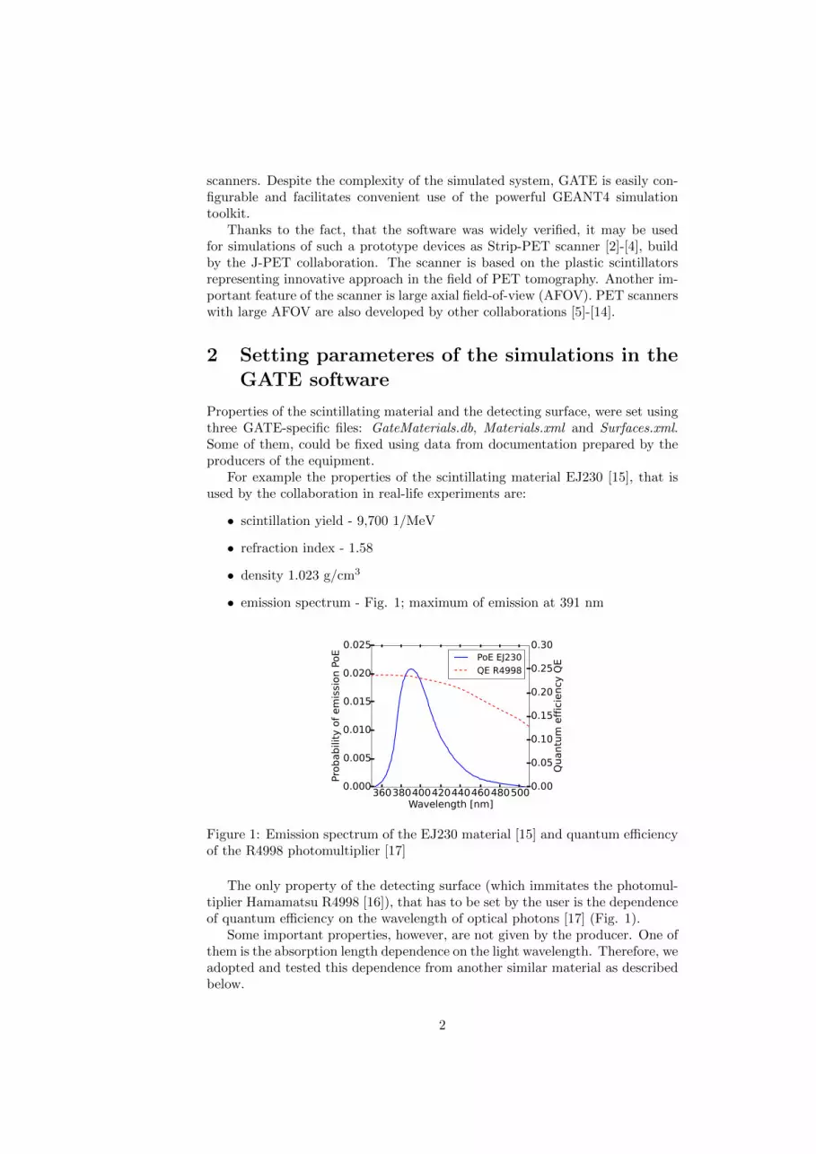
• emission spectrum - Fig. 1; maximum of emission at 391 nm
360380400420440460480500Wavelength [nm]
0.000
0.005
0.010
0.015
0.020
0.025
Probability of emission PoE
0.00
0.05
0.10
0.15
0.20
0.25
0.30
Quantum efficiency
QEPoE EJ230
QE R4998
Figure 1: Emission spectrum of the EJ230 material [15] and quantum efficiencyof the R4998 photomultiplier [17]
The only property of the detecting surface (which immitates the photomul-tiplier Hamamatsu R4998 [16]), that has to be set by the user is the dependenceof quantum efficiency on the wavelength of optical photons [17] (Fig. 1).
Some important properties, however, are not given by the producer. One ofthem is the absorption length dependence on the light wavelength. Therefore, weadopted and tested this dependence from another similar material as describedbelow.
2
2.1 Simulations of the single strip
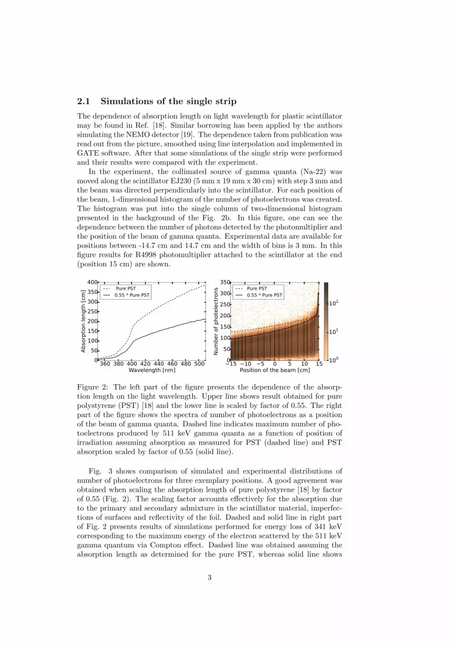
The dependence of absorption length on light wavelength for plastic scintillatormay be found in Ref. [18]. Similar borrowing has been applied by the authorssimulating the NEMO detector [19]. The dependence taken from publication wasread out from the picture, smoothed using line interpolation and implemented inGATE software. After that some simulations of the single strip were performedand their results were compared with the experiment.
In the experiment, the collimated source of gamma quanta (Na-22) wasmoved along the scintillator EJ230 (5 mm x 19 mm x 30 cm) with step 3 mm andthe beam was directed perpendicularly into the scintillator. For each position ofthe beam, 1-dimensional histogram of the number of photoelectrons was created.The histogram was put into the single column of two-dimensional histogrampresented in the background of the Fig. 2b. In this figure, one can see thedependence between the number of photons detected by the photomultiplier andthe position of the beam of gamma quanta. Experimental data are available forpositions between -14.7 cm and 14.7 cm and the width of bins is 3 mm. In thisfigure results for R4998 photomultiplier attached to the scintillator at the end(position 15 cm) are shown.
360 380 400 420 440 460 480 500Wavelength [nm]
0
50
100
150
200
250
300
350
400
Abso
rption length
[cm
] Pure PST
0.55 * Pure PST
15 10 5 0 5 10 15Position of the beam [cm]
0
50
100
150
200
250
300
350
Num
ber
of
phote
lect
rons Pure PST
0.55 * Pure PST
100
101
102
Figure 2: The left part of the figure presents the dependence of the absorp-tion length on the light wavelength. Upper line shows result obtained for purepolystyrene (PST) [18] and the lower line is scaled by factor of 0.55. The rightpart of the figure shows the spectra of number of photoelectrons as a positionof the beam of gamma quanta. Dashed line indicates maximum number of pho-toelectrons produced by 511 keV gamma quanta as a function of position ofirradiation assuming absorption as measured for PST (dashed line) and PSTabsorption scaled by factor of 0.55 (solid line).
Fig. 3 shows comparison of simulated and experimental distributions ofnumber of photoelectrons for three exemplary positions. A good agreement wasobtained when scaling the absorption length of pure polystyrene [18] by factorof 0.55 (Fig. 2). The scaling factor accounts effectively for the absorption dueto the primary and secondary admixture in the scintillator material, imperfec-tions of surfaces and reflectivity of the foil. Dashed and solid line in right partof Fig. 2 presents results of simulations performed for energy loss of 341 keVcorresponding to the maximum energy of the electron scattered by the 511 keVgamma quantum via Compton effect. Dashed line was obtained assuming theabsorption length as determined for the pure PST, whereas solid line shows
3
0 50 100 150 200 250Number of photoelectrons
0
50
100
150
200
250
300
350
Number of events
simulation
experiment
0 50 100 150 200 250Number of photoelectrons
0
50
100
150
200
250
300
Number of events
simulation
experiment
0 50 100 150 200 250Number of photoelectrons
0
100
200
300
400
500
600
Number of events
simulation
experiment
Figure 3: Comparison of the simulated and experimental histograms of energydeposited by 511 keV gamma quanta (in number of photoelectrons) for the beampositions -12 cm (left), 0 cm (middle), 12 cm (right); experimental spectrum issuppressed at low values due to the triggering conditions [2].
result after scaling the absorption by a factor of 0.55. The scaling factor wasoptimised to the experimental results.
3 Simulations of the single layer J-PET scanner
A diagnostic chamber of the J-PET detector will form a cylinder which will beconstructed from the plastic scintillator strips [20]-[22]. In this article we presentsimulations for the detector with the inner radius of R=427.8 mm (radius similarto commercially available PET systems [23], [24]). We assume that the detectorpossesses one layer build out of 384 EJ230 scintillator strips with dimensions of7 mm x 19 mm x L (L = 20 cm, 50 cm, 100 cm or 200 cm). Geometry of thesimulated scanner is visualised in Fig. 4.
Figure 4: Visualisation of the geometry of the single-layer J-PET scanner withradius of the cylinder R and the length of the scintillators L.
3.1 Scattered coincidences
In order to estimate secondary scattering of gamma quanta in the detectormaterial, we have simulated annihilations homogeneously in the 2 m long lineplaced along the central axis of the scanner. In the following, we considerfew most probable responses of the detector system (see Fig. 5). In the mostprobable case both gamma quanta will escape detection and no signal will beobserved (Nstrips = 0). The second frequent category corresponds to eventswhen only one strip was hit (Nstrips = 1). Further on for the multiplicity
4
of strips Nstrips >= 2 we can distinguish different cases for the same value ofNstrips. Therefore for the univocal description we introduce one more parameterµ. Various possibilities which may occur are listed below and depicted in Fig.5:
• Nstrips = 3, µ = −33 quanta in 3 different strips with two secondary scatterings
• Nstrips = 2, µ = −22 quanta in 2 different strips with one secondary scattering
• Nstrips = 0, µ = 0no gamma quanta registered
• Nstrips = 1, µ = 1interaction in only one strip
• Nstrips = 2, µ = 22 interactions in 2 different strips
• Nstrips = 3, µ = 33 scatterings in 3 different strips; 2 primary and 1 secondary scattering
It is also possible that there are 4, 5 or even more scatterings, depending onthe energy threshold applied to each hit.
Figure 5: Pictorial definitions of the value of multiplicity µ used further in thefollowing figures.
Histograms of the multiplicity for three different energy thresholds (0 keV,100 keV and 200 keV) and for four different lengths of scintillators (20 cm, 50 cm,100 cm and 200 cm) are presented in the Fig. 6. Results of the simulations showthat if energy threshold is set to 200 keV, there are no events where number ofhits is bigger than 2. Most of scattered coincidences (with multiplicity -2) is also
5
eliminated with this energy threshold. If the energy threshold is set to 100 keV,for lengths of scitnillators 100 cm and 200 cm, there would be even events withfour scatterings, which may negatively influence the quality of reconstructedimages.
-3 -2 0 1 2 3 4 5 6µ
10-810-710-610-510-410-310-210-1100101
Fraction of Events
L=20cm0 keV
100 keV
200 keV
-3 -2 0 1 2 3 4 5 6µ
10-810-710-610-510-410-310-210-1100101
Fraction of Events
L=50cm0 keV
100 keV
200 keV
-3 -2 0 1 2 3 4 5 6µ
10-810-710-610-510-410-310-210-1100101
Fraction of Events
L=100cm0 keV
100 keV
200 keV
-3 -2 0 1 2 3 4 5 6µ
10-810-710-610-510-410-310-210-1100101
Fraction of Events
L=200cm0 keV
100 keV
200 keV
Figure 6: Histogram of the multiplicity µ for different lengths L of the diagnosticchamber. Meanings of different values of the multiplicity µ are described in thetext and defined in Fig. 5.
For Nstrips=2 and Nstrips=3 and length of scintillators equal to L = 50 cm,histograms of time differences between subsequent hits were calculated. Thesehistograms are presented in Figs 7 - 9. Right panel of these figures show dis-tribution of difference between ID of hit modules (∆ID) as a function of hittime difference.1 The module ID increases monotonically with the grows of theazimuthal angle ϕ (see Fig. 4). Black lines in the two-dimensional histograms(Figs 7 - 10) show the boundaries between events treated as useful coincidencesand events treated as background coincidences due to the secondary scatterings.A positive value of µ (2 or 3) is assigned to events above the line, which aretreated in further analysis as true conicidences. Whereas to events below theline a negative value of µ (-3 or -2) is assigned since these events include sec-ondary scattering of gamma quanta. This boundary was used to separate eventswith different multiplicities for preparation of histograms presented in Fig. 6.
In Fig. 7, for energy thresholds 0 keV and 100 keV, in two-dimensional his-tograms there is longitudinal structure extending between points (0 ns, 0) and(3 ns, 192). These events correspond to difference between time of primary re-action of the gamma quantum in a given scintillator and a time of the secondary
1If IDs of hit modules are ID1 and ID2 then ∆ID = min(|ID1−ID2|, 384−|ID1−ID2|).
6
scattering. The larger is the angle of the primary scattered gamma quantum thelarger will be the ∆ID value and also a ∆t. For example bin with coordinates(2.9 ns, 192) corresponds to the backscattering - primary particle is backscat-tered and it is registered in the strip on the opposite side of the scintillator (2.9ns is the time needed by the gamma quanta to travel between opposite stripswith speed of light).
If the energy threshold is set to 200 keV, nearly all scattered coincidences areeliminated. In the lower panel of this figure there are results for this threshold.In ideal situation, time difference for this simulation for true coincidences wouldbe always 0 and we would have only one bin for 0 ns. Because of the fact thatgamma quanta interact with matter in different depths (Depth of Interaction),time difference is changing from 0 to about 80 ps. This picture show, what isthe time limit for time-of-flight determination with scintillator strips of 19 mmthickness.
In Fig. 8, for energy thresholds 0 keV and 100 keV, in two-dimensionalhistograms there is symmetrical butterfly-shape structure extending betweenpoints (0 ns, 0) and (3 ns, 192) and between points (3 ns, 0) and (0 ns, 192).Each event with three hits and deposited energy above the energy thresold, givestwo inputs to these histograms. An additional structure (for Nstrips = 3) whichis spanned between points (3 ns, 0) and (0 ns, 192) originates from the timedifferences between the primary interaction of one of the gamma quantum anda secondary interaction of the other or from the time difference between twosecondary interactions. Pictorial definitions of these situations are presented inFig. 5. If only the first time difference is taken into account, histograms for3 hits (Fig. 9) look like histograms for 2 hits (Fig. 7).
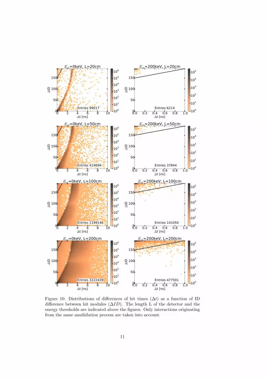
Response of the detector to the annihilations in the 2 m long line placed alongthe detector axis was simulated also for other lengths of scintillators L = 20 cm,100 cm and 200 cm. Results of these simulations for two energy thresholds(0 keV and 200 keV) are presented in Fig. 10. One can see that, the longer thescintillators, the wider the longitudal structure described above. It is causedby the fact that, the longer the scintillators, the longer the possible distancebetween places of the primary and secondary interactions. For the scannerwith 20 cm scintillators, the longest possible path along the diagonal of thelongitudinal cross-section of the scanner has length of 88 cm (∼ 2.9 ns) andfor the scanner with 200 cm scintillators, the longest possible path is equal to218 cm (7.3 ns).
7
0 1 2 3 4 5∆t [ns]
100
101
102
103
104
105
Events
Entries 414257Eth=0keV
0 1 2 3 4 5∆t [ns]
0
50
100
150
∆ID
Eth=0keV
100
101
102
103
104
105
0 1 2 3 4 5∆t [ns]
100
101
102
103
104
105
Events
Entries 139236Eth=100keV
0 1 2 3 4 5∆t [ns]
0
50
100
150
∆ID
Eth=100keV
100
101
102
103
104
105
0.00 0.05 0.10 0.15 0.20∆t [ns]
100
101
102
103
104
105
Events
Entries 37839Eth=200keV
0 1 2 3 4 5∆t [ns]
0
50
100
150
∆ID
Eth=200keV
100
101
102
103
104
105
Figure 7: Distributions of differences of hit times; Nstrips = 2, µ = −2 orµ = 2; black line in the two-dimensional histogram shows the boundary betweenevents treated as originating from primary interactions only (above the line)and events including secondary interactions (below the line). Figure presentsresults of simulations for L=50 cm. The time differences are calculated only forinteractions originating from the same annihilation process.
8
0 1 2 3 4 5∆t [ns]
100
101
102
103
104
Events
Entries 43311Eth=0keV
0 1 2 3 4 5∆t [ns]
0
50
100
150
∆ID
Eth=0keV
100
101
102
103
104
0 1 2 3 4 5∆t [ns]
100
101
102
103
104
Events
Entries 2252Eth=100keV
0 1 2 3 4 5∆t [ns]
0
50
100
150
∆ID
Eth=100keV
100
101
102
103
104
Figure 8: Distributions of differences of hit times; Nstrips=3, µ = −3 or µ = 3,both time differences are taken into account. Figure presents results of simu-lations for L=50 cm. The time differences are calculated only for interactionsoriginating from the same annihilation process. Figure is described with detailsin the text.
9
0 1 2 3 4 5∆t [ns]
100
101
102
103
104
Events
Entries 21661Eth=0keV
0 1 2 3 4 5∆t [ns]
0
50
100
150
∆ID
Eth=0keV
100
101
102
103
104
0 1 2 3 4 5∆t [ns]
100
101
102
103
104
Events
Entries 1126Eth=100keV
0 1 2 3 4 5∆t [ns]
0
50
100
150
∆ID
Eth=100keV
100
101
102
103
104
Figure 9: Distributions of differences of hit times; Nstrips=3, µ = −3 or µ = 3,only first time difference is taken into account. Figure presents results of sim-ulations for L=50 cm. The time differences are calculated only for interactionsoriginating from the same annihilation process. Figure is described with detailsin the text.
10
0 2 4 6 8 10∆t [ns]
0
50
100
150
∆ID
Entries 99017
Eth=0keV, L=20cm
100
101
102
103
104
105
106
0.0 0.2 0.4 0.6 0.8 1.0∆t [ns]
0
50
100
150
∆ID
Entries 6214
Eth=200keV, L=20cm
100
101
102
103
104
105
0 2 4 6 8 10∆t [ns]
0
50
100
150
∆ID
Entries 414694
Eth=0keV, L=50cm
100
101
102
103
104
105
106
0.0 0.2 0.4 0.6 0.8 1.0∆t [ns]
0
50
100
150
∆ID
Entries 37844
Eth=200keV, L=50cm
100
101
102
103
104
105
0 2 4 6 8 10∆t [ns]
0
50
100
150
∆ID
Entries 1199146
Eth=0keV, L=100cm
100
101
102
103
104
105
106
0.0 0.2 0.4 0.6 0.8 1.0∆t [ns]
0
50
100
150
∆ID
Entries 141050
Eth=200keV, L=100cm
100
101
102
103
104
105
0 2 4 6 8 10∆t [ns]
0
50
100
150
∆ID
Entries 3222439
Eth=0keV, L=200cm
100
101
102
103
104
105
106
0.0 0.2 0.4 0.6 0.8 1.0∆t [ns]
0
50
100
150
∆ID
Entries 477501
Eth=200keV, L=200cm
100
101
102
103
104
105
Figure 10: Distributions of differences of hit times (∆t) as a function of IDdifference between hit modules (∆ID). The length L of the detector and theenergy thresholds are indicated above the figures. Only interactions originatingfrom the same annihilation process are taken into account.
11
3.2 Accidental coincidences
An accidental coincidence is the coincidence, in which two events occur simul-taneously in a fixed time window but in fact they are independent, they comefrom different annihilations. Because of that, number of accidental coincidencesdepends on the width of the time window, the size of the detector and in contrastto the secondary scattering, the accidental coincidences depend on the activityof the source.
3.2.1 Accidental coincidences as a function of the source activity
Simulations described in this section were performed for other activities of thesource: 5 MBq, 10 MBq, 20 MBq, 30 MBq, 50 MBq, 100 MBq, 150 MBq,200 MBq, 250 MBq, 300 MBq, 350 MBq and 400 MBq. For each of these activ-ities 108 annihilations were simulated. Results of simulations for the smallest(5 MBq) and the largest (400 MBq) activity are presented in Figs 11 and 12.
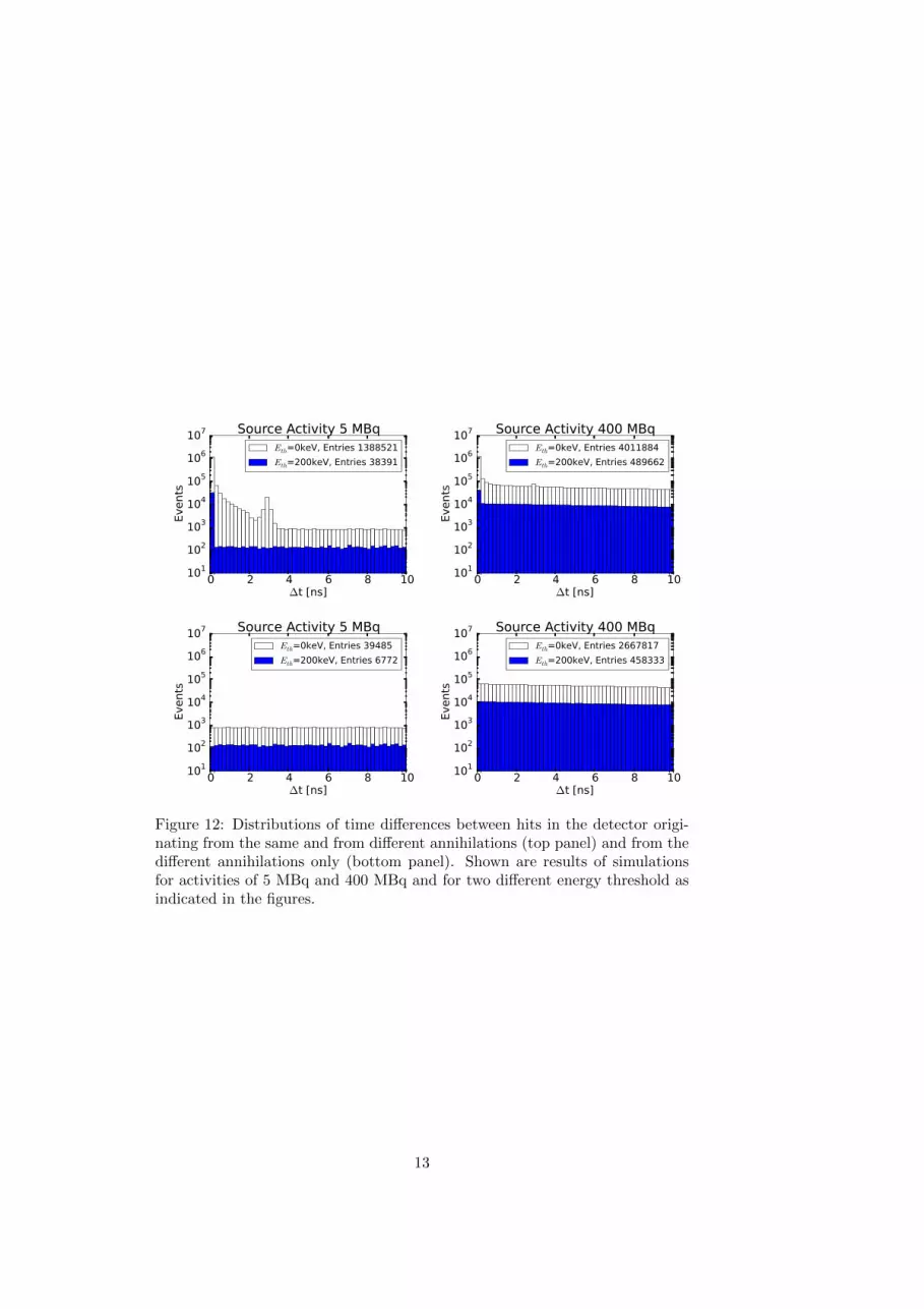
In Fig. 11 histograms contain all time differences both for hits from the sameevent and for hits from different events (there is no time window). One can seethat the first bin is higher than expected from the general exponential depen-dence. This is because this bin contains both true and accidental coincidences.The structure is better visible in Fig. 12. In the upper panel of this figure,histograms contain time differences between hits from the same and from differ-ent annihilations. If time differences from the same annihilations were omitted,there would be only accidental coincidences, as it is presented in the bottompanel of the figure.
0 10 20 30 40∆t [µs]
100101102103104105106107
Events
Source Activity 5 MBqEth=0keV,Entries 10252241
Eth=200keV,Entries 1560670
0 100 200 300 400 500∆t [ns]
100101102103104105106107
Events
Source Activity 400 MBqEth=0keV,Entries 10245339
Eth=200keV,Entries 1560820
Figure 11: Histograms of numbers of all differences of hit times for length ofscintillators equal to 50 cm, activities of 5 MBq and 400 MBq and for twodifferent energy thresholds as indicated in the legends.
12
0 2 4 6 8 10∆t [ns]
101
102
103
104
105
106
107
Events
Source Activity 5 MBqEth=0keV, Entries 1388521
Eth=200keV, Entries 38391
0 2 4 6 8 10∆t [ns]
101
102
103
104
105
106
107Events
Source Activity 400 MBqEth=0keV, Entries 4011884
Eth=200keV, Entries 489662
0 2 4 6 8 10∆t [ns]
101
102
103
104
105
106
107
Events
Source Activity 5 MBqEth=0keV, Entries 39485
Eth=200keV, Entries 6772
0 2 4 6 8 10∆t [ns]
101
102
103
104
105
106
107
Events
Source Activity 400 MBqEth=0keV, Entries 2667817
Eth=200keV, Entries 458333
Figure 12: Distributions of time differences between hits in the detector origi-nating from the same and from different annihilations (top panel) and from thedifferent annihilations only (bottom panel). Shown are results of simulationsfor activities of 5 MBq and 400 MBq and for two different energy threshold asindicated in the figures.
13
3.2.2 Accidental coincidences for time windows 3 ns and 5 ns
For simulations described in this article with the virtual linear source of annihi-lations placed along the main axis of the scanner, true coincidences are definedas two hits from the same annihilation having ∆ID vs ∆t above the black linesshown in Figs 7 - 10. Fig. 13 presents rate of such defined true coincidences asa function of annihilation source activity, time window, energy threshold, anddetector length L.
0 50 100 150 200 250 300 350 400Activity [MBq]
0100020003000400050006000700080009000
kEvents/s
Eth=0keV, Nstrips=2, µ=2
L=200cm, tw=5ns
L=200cm, tw=3ns
L=100cm, tw=5ns
L=100cm, tw=3ns
L=50cm, tw=5ns
L=50cm, tw=3ns
L=20cm, tw=5ns
L=20cm, tw=3ns
0 50 100 150 200 250 300 350 400Activity [MBq]
0
200
400
600
800
1000
1200
1400
1600
kEvents/s
Eth=200keV, Nstrips=2, µ=2
L=200cm, tw=5ns
L=200cm, tw=3ns
L=100cm, tw=5ns
L=100cm, tw=3ns
L=50cm, tw=5ns
L=50cm, tw=3ns
L=20cm, tw=5ns
L=20cm, tw=3ns
0 50 100 150 200 250 300 350 400Activity [MBq]
100
101
102
103
104
kEvents/s
Eth=0keV, Nstrips=2, µ=2
0 50 100 150 200 250 300 350 400Activity [MBq]
10-1
100
101
102
103
104
kEvents/s
Eth=200keV, Nstrips=2, µ=2
Figure 13: Simulated rate of true coincidences as a function of time window,activity and detector length. The sequence of curves in the figure is the same asin the legend (from top to bottom); bottom pictures present the same data asthe top ones but in logarithmic scale. Results for the time window of 3ns (solidlines) are indistinguishable from the results for time window of 5 ns (dashedlines).
Accidental coincidences for time windows 3 ns and 5 ns and for four lengthsof the scintillators are presented in Fig. 14. One can see that if the energythreshold is 200 keV (right column of the figure), a rate of accidental coinci-dences is reduced by the factor of about 7 in comparison to situation when thereis no energy threshold (left column of the figure).
Fig. 15 shows rate of accidental coincidences under condition that differ-ence ∆ID is larger than 96. Which means that interactions of gamma quantaoccurs in two different quarters of the cylinder (consisting of 384 scintillatorstrips). Such condition decrease the field of view of the detector to the cylinderwith radius of 30 cm, however this additional condition reduces the number ofaccidental coincidences by the factor of 2.
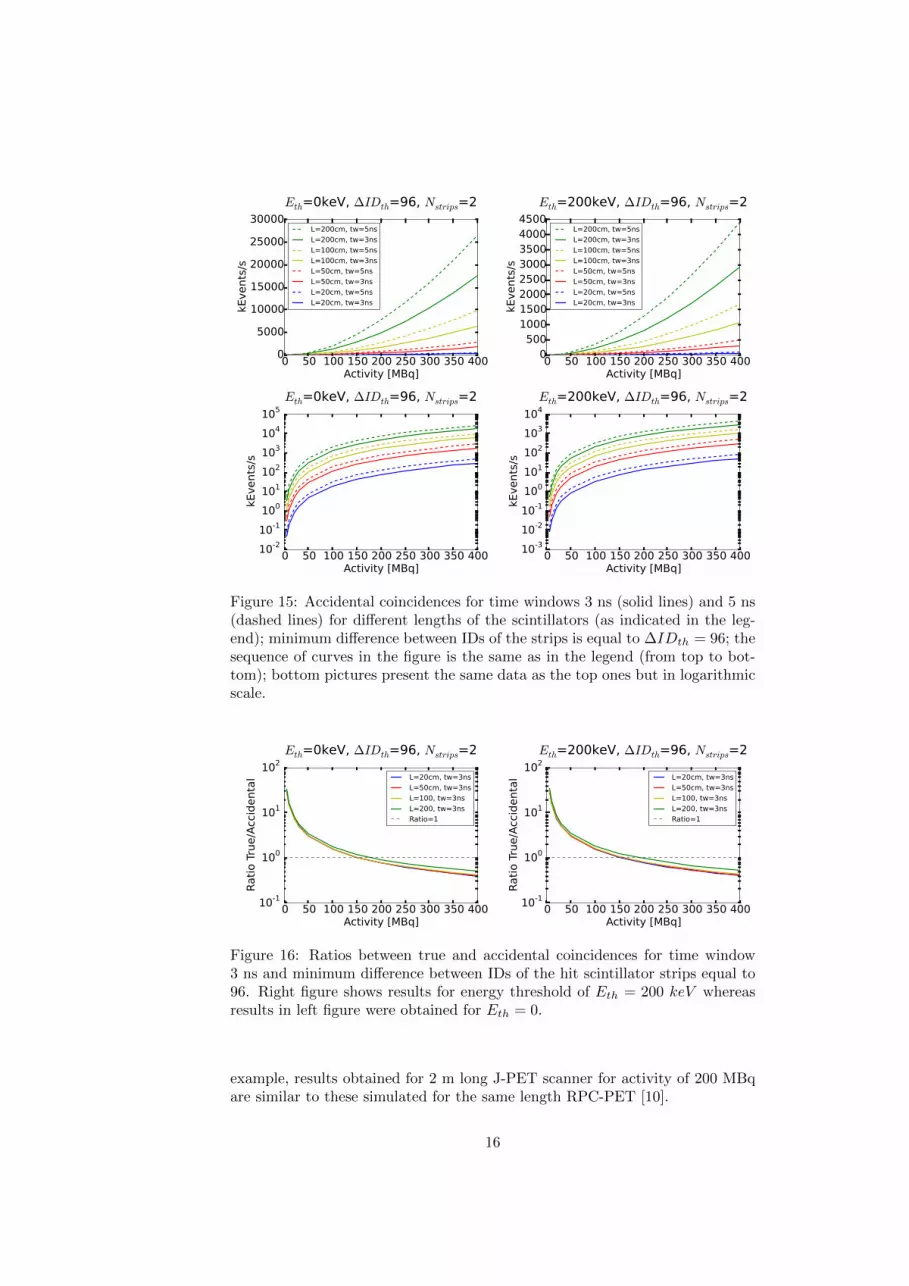
In Fig. 16 rates of true and accidental coincidences are presented. The
14
0 50 100 150 200 250 300 350 400Activity [MBq]
0
10000
20000
30000
40000
50000
60000
kEvents/s
Eth=0keV, ∆IDth=0, Nstrips=2
L=200cm, tw=5ns
L=200cm, tw=3ns
L=100cm, tw=5ns
L=100cm, tw=3ns
L=50cm, tw=5ns
L=50cm, tw=3ns
L=20cm, tw=5ns
L=20cm, tw=3ns
0 50 100 150 200 250 300 350 400Activity [MBq]
0100020003000400050006000700080009000
kEvents/s
Eth=200keV, ∆IDth=0, Nstrips=2
L=200cm, tw=5ns
L=200cm, tw=3ns
L=100cm, tw=5ns
L=100cm, tw=3ns
L=50cm, tw=5ns
L=50cm, tw=3ns
L=20cm, tw=5ns
L=20cm, tw=3ns
0 50 100 150 200 250 300 350 400Activity [MBq]
10-2
10-1
100
101
102
103
104
105
kEvents/s
Eth=0keV, ∆IDth=0, Nstrips=2
0 50 100 150 200 250 300 350 400Activity [MBq]
10-2
10-1
100
101
102
103
104
kEvents/s
Eth=200keV, ∆IDth=0, Nstrips=2
Figure 14: Accidental coincidences for time windows 3 ns (solid lines) and 5 ns(dashed lines) for different lengths of the scintillators (as indicated in the leg-end); the sequence of curves in the figure is the same as in the legend (fromtop to bottom); bottom pictures present the same data as the top ones but inlogarithmic scale.
ratio is larger for longer scintillators. It is caused by the fact that for shortscintillators there are additional accidental coincidences caused by the gammaquanta from outside of the tomograph.
4 Summary
Physical properties of the scintillating material and the photomultiplier used inthe J-PET detector were implemented in the GATE software. The simulationsprocedures were validated by the comparison of simulated and experimentalresults for the number of photoelectron spectra.
In previous research, studies of simplified Strip-PET scanner were presented[25]. Map of efficiency of 2-strip scanner was calculated and compared with thegeometrical efficiency of such a device. In present studies, background given byaccidental coincidences and multiple scattering of gamma quanta was investi-gated for single-layer 384-strip J-PET scanner.
In presented simulations, the source of annihilations was assumed to be a2 m long line placed along the main axis of the scanner. In order to compareprecisely obtained results with results for another devices, in the future thesource will be simulated in accordance with NEMA-NU-2 standard [27]. Evenso, it is possible to compare orders of magnitudes of calculated parameters. For
15
0 50 100 150 200 250 300 350 400Activity [MBq]
0
5000
10000
15000
20000
25000
30000
kEvents/s
Eth=0keV, ∆IDth=96, Nstrips=2
L=200cm, tw=5ns
L=200cm, tw=3ns
L=100cm, tw=5ns
L=100cm, tw=3ns
L=50cm, tw=5ns
L=50cm, tw=3ns
L=20cm, tw=5ns
L=20cm, tw=3ns
0 50 100 150 200 250 300 350 400Activity [MBq]
0500
10001500200025003000350040004500
kEvents/s
Eth=200keV, ∆IDth=96, Nstrips=2
L=200cm, tw=5ns
L=200cm, tw=3ns
L=100cm, tw=5ns
L=100cm, tw=3ns
L=50cm, tw=5ns
L=50cm, tw=3ns
L=20cm, tw=5ns
L=20cm, tw=3ns
0 50 100 150 200 250 300 350 400Activity [MBq]
10-210-1100101102103104105
kEvents/s
Eth=0keV, ∆IDth=96, Nstrips=2
0 50 100 150 200 250 300 350 400Activity [MBq]
10-310-210-1100101102103104
kEvents/s
Eth=200keV, ∆IDth=96, Nstrips=2
Figure 15: Accidental coincidences for time windows 3 ns (solid lines) and 5 ns(dashed lines) for different lengths of the scintillators (as indicated in the leg-end); minimum difference between IDs of the strips is equal to ∆IDth = 96; thesequence of curves in the figure is the same as in the legend (from top to bot-tom); bottom pictures present the same data as the top ones but in logarithmicscale.
0 50 100 150 200 250 300 350 400Activity [MBq]
10-1
100
101
102
Ratio True/Accidental
Eth=0keV, ∆IDth=96, Nstrips=2
L=20cm, tw=3ns
L=50cm, tw=3ns
L=100, tw=3ns
L=200, tw=3ns
Ratio=1
0 50 100 150 200 250 300 350 400Activity [MBq]
10-1
100
101
102
Ratio True/Accidental
Eth=200keV, ∆IDth=96, Nstrips=2
L=20cm, tw=3ns
L=50cm, tw=3ns
L=100, tw=3ns
L=200, tw=3ns
Ratio=1
Figure 16: Ratios between true and accidental coincidences for time window3 ns and minimum difference between IDs of the hit scintillator strips equal to96. Right figure shows results for energy threshold of Eth = 200 keV whereasresults in left figure were obtained for Eth = 0.
example, results obtained for 2 m long J-PET scanner for activity of 200 MBqare similar to these simulated for the same length RPC-PET [10].
16
Acknowledgements
We acknowledge technical and administrative support by T. Gucwa-Rys, A. Heczko,M. Kajetanowicz, G. Konopka-Cupia l, W. Migda l, and the financial supportby the Polish National Center for Development and Research through grantINNOTECH-K1/IN1/64/159174/NCBR/12, the Foundation for Polish Sciencethrough MPD programme, the EU and MSHE Grant No. POIG.02.03.00-16100-013/09, Doctus the Lesser Poland PhD Scholarship Fund and Marian Smolu-chowski Krakow Research Consortium ”Matter-Energy-Future”.
References
[1] S. Jan et al., Physics in medicine and biology 49.19, 4543 (2004).
[2] P. Moskal et al., Nucl. Instrum. Meth. A 764, 317 (2014), arXiv:1407.7395[physics.ins-det].
[3] P. Moskal et al., Nucl. Instrum. Meth. A 775, 54 (2015), arXiv:1412.6963[physics.ins-det].
[4] L. Raczynski et al., Nucl. Instr. and Meth. A 764, 186 (2014),arXiv:1407.8293 [physics.ins-det].
[5] I. Insaini et al., Nuclear Science Symposium and Medical Imaging Conference(NSS/MIC), 2013 IEEE, 1 (2013).
[6] D. R. DeGrado et al., Journal of Nuclear Medicine, 35.8, 1398 (1994).
[7] W. C. Hunter et al., Nuclear Science Symposium Conference Record(NSS/MIC), 2009 IEEE, 3900 (2009).
[8] M. Couceiro, et al., Nucl. Instr. and Meth. A, 580.1, 485 (2007).
[9] E. Yoshida, et al., Nuclear Science Symposium Conference Record(NSS/MIC), 2009 IEEE, 3628 (2009).
[10] E. Yoshida, et al., Nucl. Instr. and Meth. A, 621.1, 576 (2010).
[11] J. L. Lacy, et al., Nucl. Instr. and Meth. A, 471.1, 88 (2001).
[12] N. N. Shehad, et al., Nuclear Science Symposium Conference Record, 2005IEEE, 5, 2895 (2005).
[13] G. Belli, et al., Journal of Physics: Conference Series, 41.1, 555 (2006).
[14] A. Blanco, et al., Nucl. Instr. and Meth. A, 602.3, 780 (2009).
[15] Eljen Technology, EJ230 Data Sheet, available at:www.eljentechnology.comindex.phpproductsplastic-scintillators65-ej-228.
[16] Hamamatsu, R4998 Data Sheet, available at:http:www.hamamatsu.comresourcespdfetdR4998 TPMH1261E02.pdf.