11th International Conference on Urban Drainage, Edinburgh, Scotland, UK, 2008

Modelling of Priority Pollutants releases from Urban Areas

W. De Keyser, V. Gevaert, F. Verdonck and L. Benedetti*

BIOMATH, Ghent University, Coupure Links 653, 9000 Ghent, Belgium

*corresponding author: Lorenzo.Benedetti@ugent.be, +32 9 264 5937

ABSTRACT In the framework of the EU project ScorePP (Source Control Options for Reducing Emissions of Priority Pollutants), dynamic PPs (priority pollutants) fate models are being developed to assess appropriate strategies for limiting the release of PPs from urban sources and for treating PPs on a variety of spatial scales. Different possible sources of PP releases were mapped and both their release pattern and their loads were quantified as detailed as possible. This paper focuses on the link between the gathered PP sources data and the dynamic models of the urban environment. This link consists of: (1) a method for the quantitative and structured storage of temporal emission pattern information, (2) the coupling of GIS-based spatial emission source data with temporal emission pattern information and (3) the generation of PP release time series to feed the dynamic sewer catchment model. Steps 2 and 3 were included as the main features of a dedicated software tool. Finally, this paper also illustrates the method’s applicability to generate model input timeseries for generic pollutants (N, P and COD/BOD) in addition to priority pollutants. KEYWORDS Emission pattern; time series; priority pollutants; release dynamics; sewer catchment model INTRODUCTION Priority pollutants and the ScorePP project The objectives of the EU project ScorePP (Source Control Options for Reducing Emissions of Priority Pollutants, www.scorepp.eu) are to identify the sources of PPs in urban areas and to identify and assess appropriate strategies for limiting the release of PPs from urban sources and for treating PPs on a variety of spatial scales. To this purpose, integrated dynamic urban scale source-and-flux models are developed for quantifying the release of PPs from urban sources, the fate of PPs within different treatment systems implemented on a variety of scales, substance flows and behaviour within the urban drainage and wastewater system and, consequently, their emissions to the aquatic environment. The models can be used for quantifying the release of PPs from urban sources and the fate of PPs within different treatment systems. An integrated, dynamic model is able to predict the fate of PPs and therefore assess the compliance with Environmental Quality Standards (EQSs) which need to be established. The model enables “what-if” scenarios with comparison of the effect and efficiency of different emission barriers (alternative technologies, management options and substitution options) before decisions are made.

De Keyser et al. 1

11th International Conference on Urban Drainage, Edinburgh, Scotland, UK, 2008 The focus of this paper is on the quantitative description of the loads and dynamics of the PP sources at any stage of a substance’s life cycle by means of models of PP releases, which are used to feed the integrated model. Depending on the available information on PP sources, deterministic, stochastic or both modelling techniques need to be used. Phenomenological modelling of PP inputs to the urban catchment In literature, different techniques can be found to generate a dynamic model input. For the Benchmark Simulation Model N°2, a WWTP influent wastewater generator used by Jeppsson et al. (2006) included four entities: (1) diurnal phenomena modelled using a second-order harmonic function, (2) seasonal phenomena, (3) weekend effects and (4) holiday effects, the last two modelled with lower flow rates and pollutant loads. Because this generator directly modelled the treatment plant influent, urban drainage phenomena like groundwater infiltration, rain and storm weather and first flush events were included. In this paper, however, the aim is not to model only the WWTP but the whole urban catchment. The WWTP influent is therefore generated in the model itself. A second substantial difference between most influent generators found in literature and the approach presented here, is that the focus is not on hydrodynamics and on the “generic” pollutants N, P, COD and BOD, but rather on modelling the release of prioritary pollutants by different sources in an urban catchment, having different characteristics than the generic pollutants. An example of detailed mechanistic modelling can be found in Ort (2006), where benzo-triazole was traced and measured in a Swiss sewer catchment to validate the modelling of discharges by household dishwashers. The discharge activity of the individual dishwashers was modelled as block shaped peaks that transform to Gaussian peak shaped pulses when they are transported in the sewer network. The occurrence time of the discharge and the initial discharge duration were randomly sampled from certain intervals. As the discharges only took about 1 to 2 minutes, the temporal resolution used in this study was maximum 1 minute. Such high frequency is not needed for the modelling of PP fate and concentrations in a catchment over a period of several years. However, the concept of modelling individual random peaks and then summing all individual time series to obtain an overall release pattern for all facilities in a (sub)catchment was adopted. METHODS Emission Strings Different possibilities can be thought of to map PP release sources. For example, a substance could be followed from cradle to grave, estimating in each lifecycle step the emissions of the PP to the different receiving compartments of the environment, together with its characteristic release pattern. This “lifecycle analysis” approach, as was suggested in the Technical Guidance Document on Risk Assessment (European Commission, 2003), minimises the risk of unintentionally omitting certain PP release sources. On the other hand, the practical applicability of the proposed methodology would be highly increased using a source classification system that is compatible with the existing local GIS-based emission registers of municipalities, as the scope of the ScorePP project is limited to the urban environment. Therefore it was decided that the lifecycle approach could be used for data gathering purposes, but the possible PP sources would finally be identified by the unique

2 Modelling of Priority Pollutants releases from Urban Areas

11th International Conference on Urban Drainage, Edinburgh, Scotland, UK, 2008

combination of a CAS1, NACE2 and NOSE-P3 classification code, pointing out respectively the chemical identification of the PP, and the activity and process in which the chemical is released into the environment. This combination of CAS, NACE and NOSE-P classification codes, together with the expected emission pattern and the receiving compartment, was called an ‘emission string’. Generic emission data on the possible urban sources of 26 PPs was collected and stored in a central database. Storage of temporal emission pattern information A method was developed for the structured storage of quantitative release dynamics in a database. Natural release dynamics show diurnal and seasonal variations. However, releases which are influenced by human behaviour show three characteristic properties: daily, weekly and yearly patterns. Diurnal effects are included in the daily pattern, which describes how the PP release fluctuates during a 24 hour period. The weekly pattern takes into account phenomena like the “weekend effect”. The yearly pattern describes the fluctuations in PP release magnitude due to e.g. seasonal variations or “holiday effects”. Moreover, a “multiyear” pattern was implemented, to reproduce e.g. the decision to phase out the production or use of certain chemicals over a period of several years. A similar approach of multiplying a daily, weekly and yearly pattern to generate a typical household wastewater flow rate pattern can be found in Gernaey et al. (2005). To describe this dynamic behaviour, a thorough literature review was performed, resulting in a list of 24 daily patterns, 11 weekly patterns and 14 yearly patterns. Each pattern has its own set of parameters, for which default values are proposed. As some patterns only differ from each other in their default parameter values, they can be summarised in these more generic main categories: • Daily patterns:

o Constant release during a certain period of the day o Block pattern, alternating periods of emission / no emission o Peak emission, followed by a decline to a lower level of constant release o Two distinct emission peaks, followed by a decline to a lower level of constant release o n random emission peaks on moments sampled from a distribution o One, two or three emission peaks at a specified moment with a specified duration o Diurnal release pattern (day/night)

• Weekly patterns:

o Continuous release o Workday/weekend pattern o Workday/weekend pattern with no release on one day o Release on one day o Release on some days, with different magnitude during weekends o Release on random day(s) sampled from a distribution

1 Chemical Abstracts Service registry number 2 Nomenclature statistique des Activités économiques dans la Communauté Européenne (European standard

nomenclature for economic activities) 3 NOmenclature for Sources of Emissions – Process

De Keyser et al. 3

11th International Conference on Urban Drainage, Edinburgh, Scotland, UK, 2008

• Yearly patterns: o Continuous release o Continuous release pattern with no release during a period o Continuous release pattern with decreased release during a period o Continuous release pattern with decreased release during 2 independent sets of weeks o Continuous release from a start week to an end week o Release in random week(s) sampled from a distribution

As the multiyear pattern was considered to be mainly a result of policy, only two patterns were distinguished: stationary yearly loads or linear change in pollutant loads over a number of years. The total pattern description has the shape of a four-element vector of the format [D,W,Y,M], in which D is the daily pattern identifier, W the weekly, Y the yearly and M the multiyear. The required set of pattern-specific parameters is also stored in the database in a defined vector format. To facilitate this database input, a graphical user interface was designed which allows the user to pick the pattern from a drop-down menu and adjust the associated parameter values in a table. To provide more flexibility, also linear combinations of up to four patterns can be used. To build a custom pattern vector, either expert knowledge about the emission process can be used, or experimental measurement campaign data. As literature on release dynamics of priority pollutants is scarce, assumptions on the shape of a pattern will often need to be made. In some exceptional cases where there is neither data nor knowledge about the release dynamics, a continuous release pattern is chosen. Of course, this limits the benefits of dynamic modelling and should thus be avoided whenever possible. Stochasticity Most of the release patterns described above are deterministic. This means that the PP release is defined both in time and magnitude. E.g. when a pattern with an alternation of release and no release is assigned to a certain emission string, the magnitude of the PP release and the points in time on which the release starts and stops will be equal every time the pattern is repeated. For some industrial cyclic batch processes this will be the case, but in many other situations this deterministic behaviour does not resemble reality. Therefore, randomness or stochasticity was introduced in two ways. The first method was the addition of random noise to the obtained timeseries (applied in e.g. Gernaey et al., 2005). White Gaussian noise can be generated on every time step as a random number sampled from a normal distribution N(µ,σ²) with mean zero and standard deviation σ equal to one third of a defined noise magnitude. Like this, 99.7% of the sampled noise values will lie within the specified noise magnitude of 3σ. The second way followed to obtain more stochastic timeseries was to allow some pattern parameters to be randomly sampled from a specified range or distribution. An example is a diurnal pattern in which the times to switch from day into night and vice versa are randomly sampled from (uniform) distributions instead of having a fixed parameter value. Development of a model input generator To automate the generation of dynamic model input timeseries, a software tool was developed which has the following functionalities:

4 Modelling of Priority Pollutants releases from Urban Areas

11th International Conference on Urban Drainage, Edinburgh, Scotland, UK, 2008

• combination into an overall emission table of (1) generic emission string information on possible PP sources and their default release patterns with (2) case specific data on PP releasing facilities and their pollutant loads present in the catchment;

• a graphical user interface for easy editing of the tables and emission pattern vectors; • for each facility in the emission table: generation of a release time series (with a user

specified temporal resolution) according to the release pattern vector and the associated parameter vector;

• application of normal distributed noise on the obtained timeseries; • scaling of the time series to match the facility’s yearly pollutant load; • clustering of time series based on user specified characteristics (e.g. PP, source type,

sub-catchment, …); • saving the generated time series in files which can directly be fed to the integrated

catchment model in the WEST modelling and simulation software (MOST4Water, Kortrijk; Vanhooren et al., 2003);

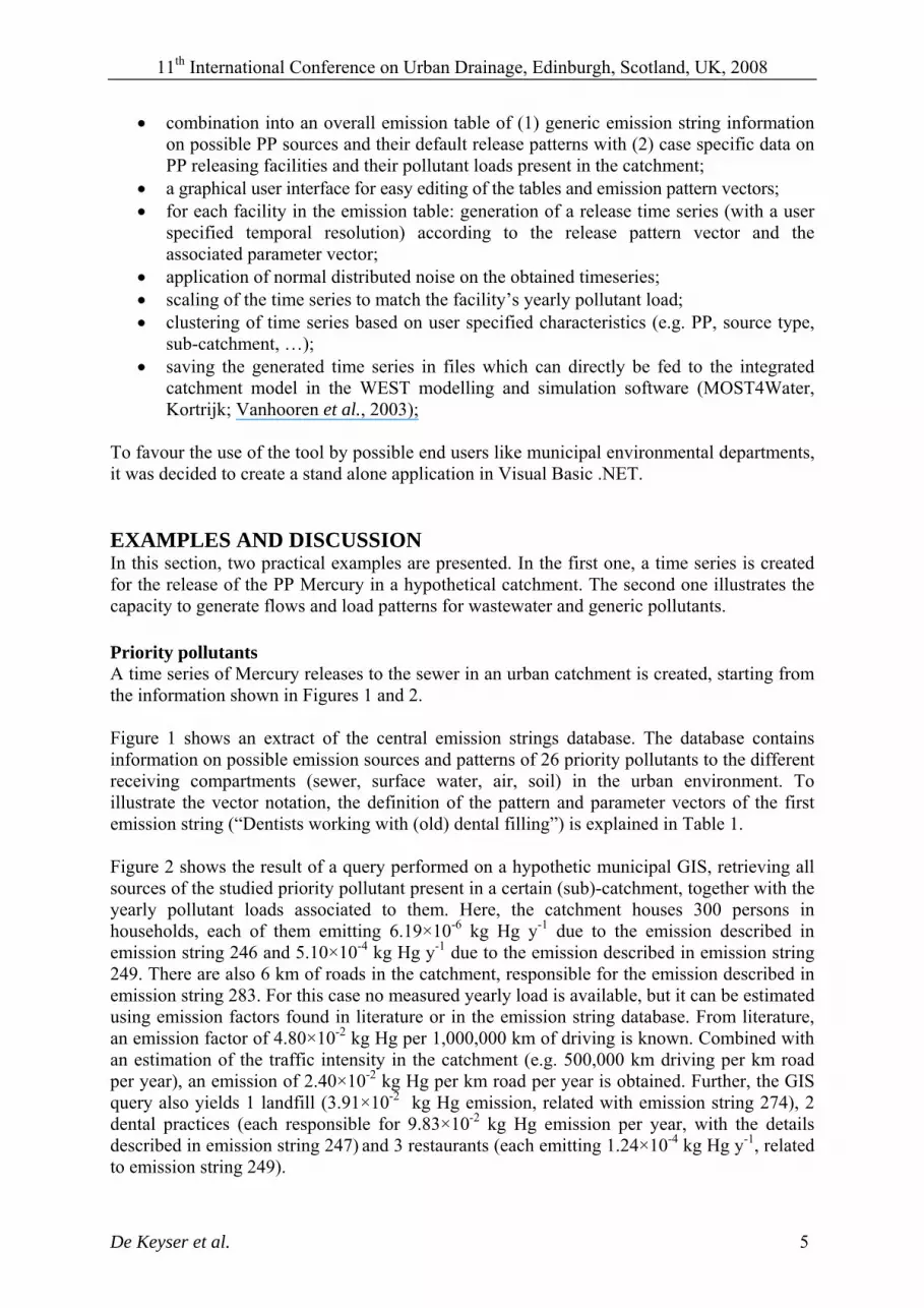
To favour the use of the tool by possible end users like municipal environmental departments, it was decided to create a stand alone application in Visual Basic .NET. EXAMPLES AND DISCUSSION In this section, two practical examples are presented. In the first one, a time series is created for the release of the PP Mercury in a hypothetical catchment. The second one illustrates the capacity to generate flows and load patterns for wastewater and generic pollutants. Priority pollutants A time series of Mercury releases to the sewer in an urban catchment is created, starting from the information shown in Figures 1 and 2. Figure 1 shows an extract of the central emission strings database. The database contains information on possible emission sources and patterns of 26 priority pollutants to the different receiving compartments (sewer, surface water, air, soil) in the urban environment. To illustrate the vector notation, the definition of the pattern and parameter vectors of the first emission string (“Dentists working with (old) dental filling”) is explained in Table 1. Figure 2 shows the result of a query performed on a hypothetic municipal GIS, retrieving all sources of the studied priority pollutant present in a certain (sub)-catchment, together with the yearly pollutant loads associated to them. Here, the catchment houses 300 persons in households, each of them emitting 6.19×10-6 kg Hg y-1 due to the emission described in emission string 246 and 5.10×10-4 kg Hg y-1 due to the emission described in emission string 249. There are also 6 km of roads in the catchment, responsible for the emission described in emission string 283. For this case no measured yearly load is available, but it can be estimated using emission factors found in literature or in the emission string database. From literature, an emission factor of 4.80×10-2 kg Hg per 1,000,000 km of driving is known. Combined with an estimation of the traffic intensity in the catchment (e.g. 500,000 km driving per km road per year), an emission of 2.40×10-2 kg Hg per km road per year is obtained. Further, the GIS query also yields 1 landfill (3.91×10-2 kg Hg emission, related with emission string 274), 2 dental practices (each responsible for 9.83×10-2 kg Hg emission per year, with the details described in emission string 247) and 3 restaurants (each emitting 1.24×10-4 kg Hg y-1, related to emission string 249).

De Keyser et al. 5

11th International Conference on Urban Drainage, Edinburgh, Scotland, UK, 2008 ES_ID NACE NOSE-P Description Default pattern Default parameters

247 85.13 111.03.02 Dentists working with (old) dental filling [10,6,2,1] [[8:30,19,10,1.00,block,0:01],[[6,7]],[[1,30,31,32]],[]]

246 - - Dental amalgam filling [24,1,1,1] [[[1,1,1,1,1,2,8,10,9,6,4,3,3,2,2,2,3,3,4,6,8,8,4,1],5,1, block,0:01],[],[],[]]

249 - 113.01 Food handling and consumption [10,5,1,1] [[6,23,3,1.00,block,0:10],[2,3],[],[]]

258 31.40 105.13.01 Manufacture of primary batteries [1,1,2,1] [[],[],[[1,30,31,32,52]],[]]

270 17.00 105.4 Pre-treatment of fibres or textiles [1,1,2,1] [[],[],[[1,30,31,32,33,34,52]],[]]

271 23.10 104.08.01 Coke ovens [1,1,1,1] [[],[],[],[]]

274 90.00 109.06 Leachate from landfills (to sewer after on site treatment) [1,1,1,1] [[],[],[],[]]

257 24.00 105.09 Processes in the chlor-alkali industry [1,1,3,1] [[],[],[[1,30,31,32,33,34,52],0.75],[]]

273 15.10 105.03.42 Slaughter houses (effluent of on site treatment plant) [3,6,3,1] [[7,18],[[6,7]],[[1,30,31,32,33,34,52],0.5],[]]

283 60.20 201 Erosion of tires [17,6,3,1][23,1,1,1] [[7,8,9,15,17,19,1.00,triangular],[[6,7]],[[1,30,31,32,33,34,52],0.75]][[6,23,3.00,1],[],[]]

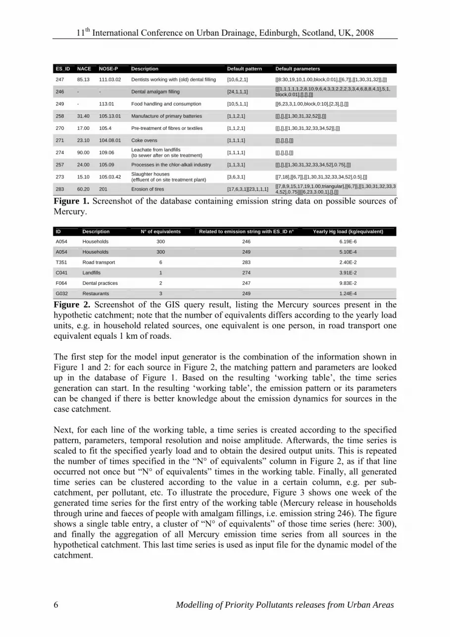
Figure 1. Screenshot of the database containing emission string data on possible sources of Mercury. ID Description N° of equivalents Related to emission string with ES_ID n° Yearly Hg load (kg/equivalent)

A054 Households 300 246 6.19E-6

A054 Households 300 249 5.10E-4

T351 Road transport 6 283 2.40E-2

C041 Landfills 1 274 3.91E-2

F064 Dental practices 2 247 9.83E-2

G032 Restaurants 3 249 1.24E-4

Figure 2. Screenshot of the GIS query result, listing the Mercury sources present in the hypothetic catchment; note that the number of equivalents differs according to the yearly load units, e.g. in household related sources, one equivalent is one person, in road transport one equivalent equals 1 km of roads. The first step for the model input generator is the combination of the information shown in Figure 1 and 2: for each source in Figure 2, the matching pattern and parameters are looked up in the database of Figure 1. Based on the resulting ‘working table’, the time series generation can start. In the resulting ‘working table’, the emission pattern or its parameters can be changed if there is better knowledge about the emission dynamics for sources in the case catchment. Next, for each line of the working table, a time series is created according to the specified pattern, parameters, temporal resolution and noise amplitude. Afterwards, the time series is scaled to fit the specified yearly load and to obtain the desired output units. This is repeated the number of times specified in the “N° of equivalents” column in Figure 2, as if that line occurred not once but “N° of equivalents” times in the working table. Finally, all generated time series can be clustered according to the value in a certain column, e.g. per sub-catchment, per pollutant, etc. To illustrate the procedure, Figure 3 shows one week of the generated time series for the first entry of the working table (Mercury release in households through urine and faeces of people with amalgam fillings, i.e. emission string 246). The figure shows a single table entry, a cluster of “N° of equivalents” of those time series (here: 300), and finally the aggregation of all Mercury emission time series from all sources in the hypothetical catchment. This last time series is used as input file for the dynamic model of the catchment.

6 Modelling of Priority Pollutants releases from Urban Areas

11th International Conference on Urban Drainage, Edinburgh, Scotland, UK, 2008

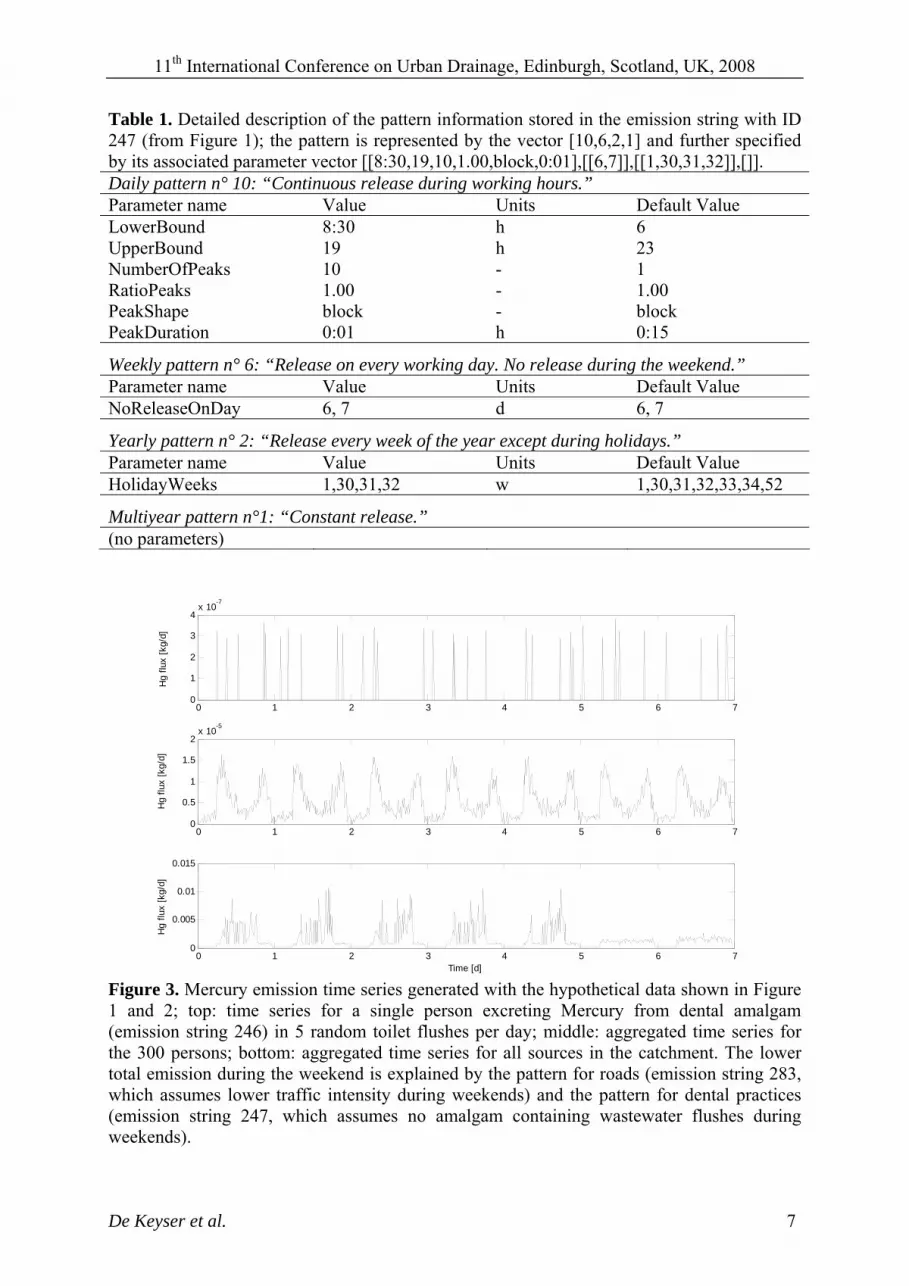
Table 1. Detailed description of the pattern information stored in the emission string with ID 247 (from Figure 1); the pattern is represented by the vector [10,6,2,1] and further specified by its associated parameter vector [[8:30,19,10,1.00,block,0:01],[[6,7]],[[1,30,31,32]],[]]. Daily pattern n° 10: “Continuous release during working hours.” Parameter name Value Units Default Value LowerBound 8:30 h 6 UpperBound 19 h 23 NumberOfPeaks 10 - 1 RatioPeaks 1.00 - 1.00 PeakShape block - block PeakDuration 0:01 h 0:15

Weekly pattern n° 6: “Release on every working day. No release during the weekend.” Parameter name Value Units Default Value NoReleaseOnDay 6, 7 d 6, 7

Yearly pattern n° 2: “Release every week of the year except during holidays.” Parameter name Value Units Default Value HolidayWeeks 1,30,31,32 w 1,30,31,32,33,34,52

Multiyear pattern n°1: “Constant release.” (no parameters)

0 1 2 3 4 5 6 70

1

2

3

4x 10-7

Hg

flux

[kg/

d]

0 1 2 3 4 5 6 70

0.5

1

1.5

2x 10-5

Hg

flux

[kg/

d]

0 1 2 3 4 5 6 70

0.005

0.01

0.015

Time [d]

Hg

flux

[kg/

d]

Figure 3. Mercury emission time series generated with the hypothetical data shown in Figure 1 and 2; top: time series for a single person excreting Mercury from dental amalgam (emission string 246) in 5 random toilet flushes per day; middle: aggregated time series for the 300 persons; bottom: aggregated time series for all sources in the catchment. The lower total emission during the weekend is explained by the pattern for roads (emission string 283, which assumes lower traffic intensity during weekends) and the pattern for dental practices (emission string 247, which assumes no amalgam containing wastewater flushes during weekends).

De Keyser et al. 7

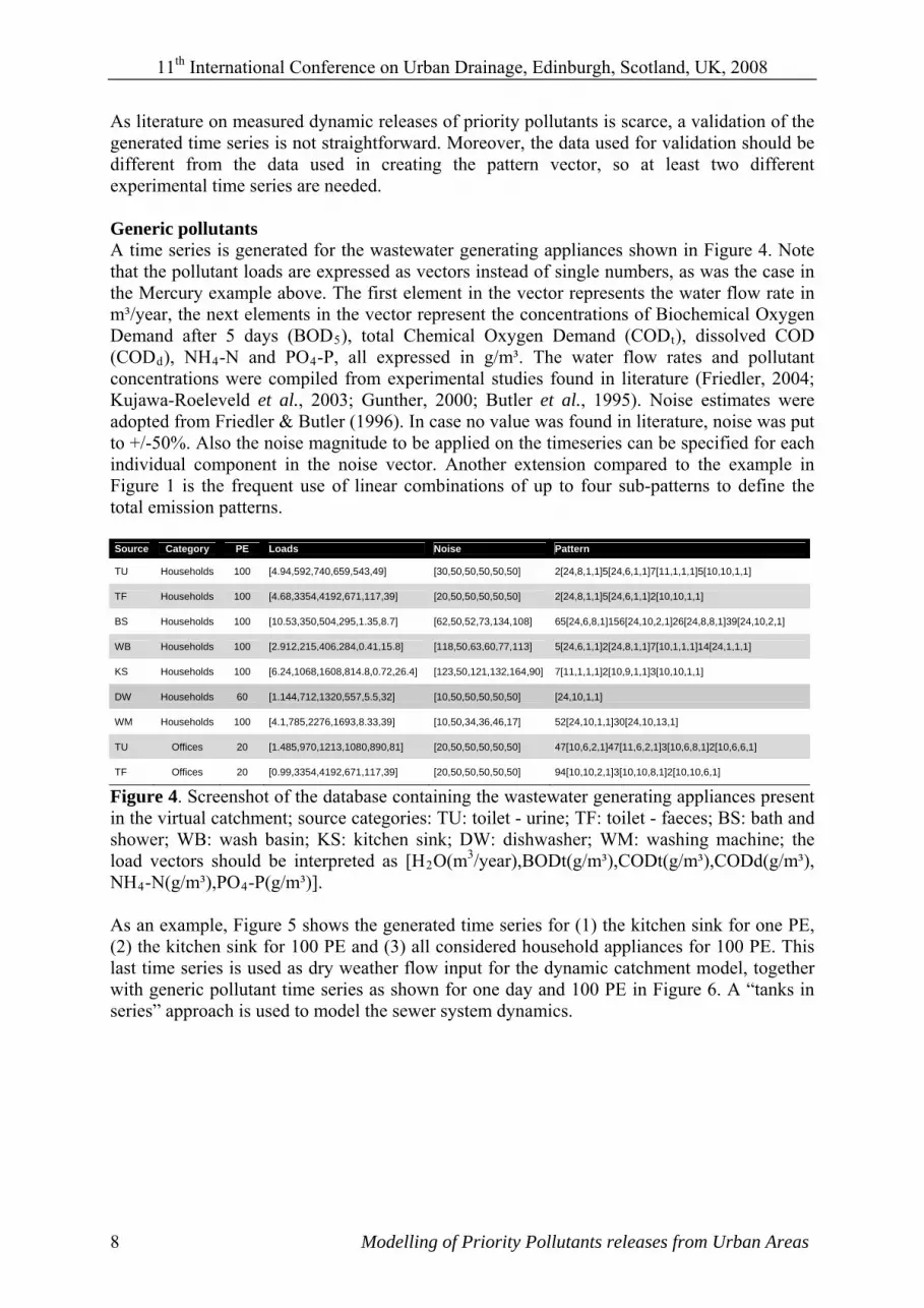
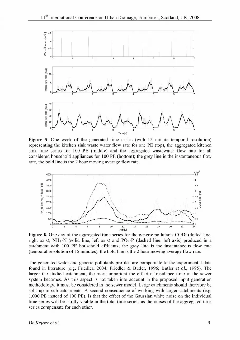
11th International Conference on Urban Drainage, Edinburgh, Scotland, UK, 2008 As literature on measured dynamic releases of priority pollutants is scarce, a validation of the generated time series is not straightforward. Moreover, the data used for validation should be different from the data used in creating the pattern vector, so at least two different experimental time series are needed. Generic pollutants A time series is generated for the wastewater generating appliances shown in Figure 4. Note that the pollutant loads are expressed as vectors instead of single numbers, as was the case in the Mercury example above. The first element in the vector represents the water flow rate in m³/year, the next elements in the vector represent the concentrations of Biochemical Oxygen Demand after 5 days (BOD5), total Chemical Oxygen Demand (CODt), dissolved COD (CODd), NH4-N and PO4-P, all expressed in g/m³. The water flow rates and pollutant concentrations were compiled from experimental studies found in literature (Friedler, 2004; Kujawa-Roeleveld et al., 2003; Gunther, 2000; Butler et al., 1995). Noise estimates were adopted from Friedler & Butler (1996). In case no value was found in literature, noise was put to +/-50%. Also the noise magnitude to be applied on the timeseries can be specified for each individual component in the noise vector. Another extension compared to the example in Figure 1 is the frequent use of linear combinations of up to four sub-patterns to define the total emission patterns. Source Category PE Loads Noise Pattern

TU Households 100 [4.94,592,740,659,543,49] [30,50,50,50,50,50] 2[24,8,1,1]5[24,6,1,1]7[11,1,1,1]5[10,10,1,1]

TF Households 100 [4.68,3354,4192,671,117,39] [20,50,50,50,50,50] 2[24,8,1,1]5[24,6,1,1]2[10,10,1,1]

BS Households 100 [10.53,350,504,295,1.35,8.7] [62,50,52,73,134,108] 65[24,6,8,1]156[24,10,2,1]26[24,8,8,1]39[24,10,2,1]

WB Households 100 [2.912,215,406,284,0.41,15.8] [118,50,63,60,77,113] 5[24,6,1,1]2[24,8,1,1]7[10,1,1,1]14[24,1,1,1]

KS Households 100 [6.24,1068,1608,814.8,0.72,26.4] [123,50,121,132,164,90] 7[11,1,1,1]2[10,9,1,1]3[10,10,1,1]

DW Households 60 [1.144,712,1320,557,5.5,32] [10,50,50,50,50,50] [24,10,1,1]

WM Households 100 [4.1,785,2276,1693,8.33,39] [10,50,34,36,46,17] 52[24,10,1,1]30[24,10,13,1]

TU Offices 20 [1.485,970,1213,1080,890,81] [20,50,50,50,50,50] 47[10,6,2,1]47[11,6,2,1]3[10,6,8,1]2[10,6,6,1]

TF Offices 20 [0.99,3354,4192,671,117,39] [20,50,50,50,50,50] 94[10,10,2,1]3[10,10,8,1]2[10,10,6,1]

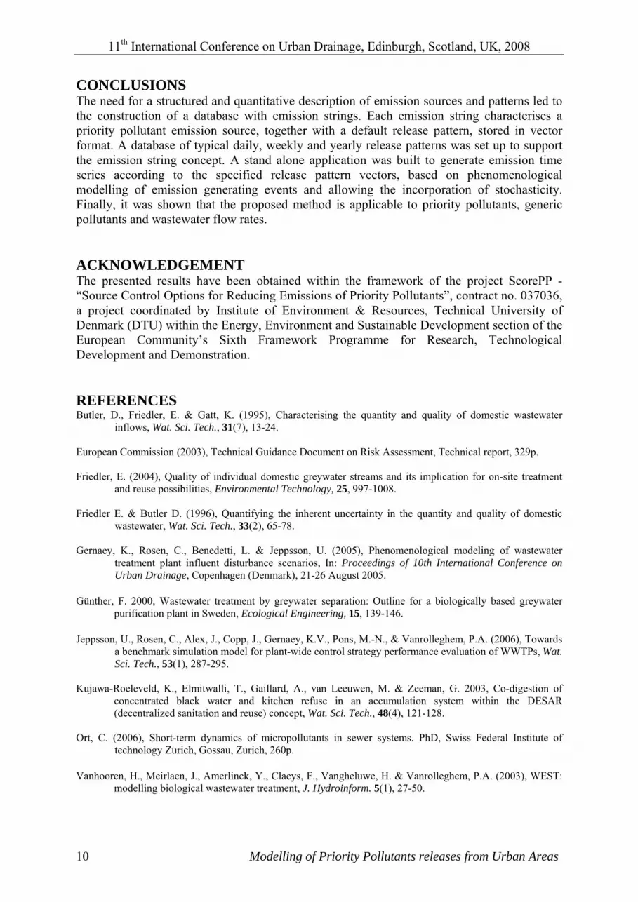
Figure 4. Screenshot of the database containing the wastewater generating appliances present in the virtual catchment; source categories: TU: toilet - urine; TF: toilet - faeces; BS: bath and shower; WB: wash basin; KS: kitchen sink; DW: dishwasher; WM: washing machine; the load vectors should be interpreted as [H2O(m3/year),BODt(g/m³),CODt(g/m³),CODd(g/m³), NH4-N(g/m³),PO4-P(g/m³)]. As an example, Figure 5 shows the generated time series for (1) the kitchen sink for one PE, (2) the kitchen sink for 100 PE and (3) all considered household appliances for 100 PE. This last time series is used as dry weather flow input for the dynamic catchment model, together with generic pollutant time series as shown for one day and 100 PE in Figure 6. A “tanks in series” approach is used to model the sewer system dynamics.

8 Modelling of Priority Pollutants releases from Urban Areas

11th International Conference on Urban Drainage, Edinburgh, Scotland, UK, 2008

0 1 2 3 4 5 6 70

0.5

1

1.5

Wat

er fl

ow ra

te [m

³/d]

0 1 2 3 4 5 6 70

5

10

Wat

er fl

ow ra

te [m

³/d]

0 1 2 3 4 5 6 70

10

20

30

40

Wat

er fl

ow ra

te [m

³/d]

Time [d] Figure 5. One week of the generated time series (with 15 minute temporal resolution) representing the kitchen sink waste water flow rate for one PE (top), the aggregated kitchen sink time series for 100 PE (middle) and the aggregated wastewater flow rate for all considered household appliances for 100 PE (bottom); the grey line is the instantaneous flow rate, the bold line is the 2 hour moving average flow rate.

0 2 4 6 8 10 12 14 16 18 20 22 240

0.5

1

1.5

2

2.5

3

3.5

4

4.5x 104

CO

Dt l

oad

[g/d

]

time [d]0 2 4 6 8 10 12 14 16 18 20 22 24

0

500

1000

1500

2000

2500

3000

3500

4000

4500

NH

4-N a

nd P

O4-P

load

[g/d

]

time [d] Figure 6. One day of the aggregated time series for the generic pollutants CODt (dotted line, right axis), NH4-N (solid line, left axis) and PO4-P (dashed line, left axis) produced in a catchment with 100 PE household effluents; the grey line is the instantaneous flow rate (temporal resolution of 15 minutes), the bold line is the 2 hour moving average flow rate. The generated water and generic pollutants profiles are comparable to the experimental data found in literature (e.g. Friedler, 2004; Friedler & Butler, 1996; Butler et al., 1995). The larger the studied catchment, the more important the effect of residence time in the sewer system becomes. As this aspect is not taken into account in the proposed input generation methodology, it must be considered in the sewer model. Large catchments should therefore be split up in sub-catchments. A second consequence of working with larger catchments (e.g. 1,000 PE instead of 100 PE), is that the effect of the Gaussian white noise on the individual time series will be hardly visible in the total time series, as the noises of the aggregated time series compensate for each other.

De Keyser et al. 9

11th International Conference on Urban Drainage, Edinburgh, Scotland, UK, 2008

10 Modelling of Priority Pollutants releases from Urban Areas

CONCLUSIONS The need for a structured and quantitative description of emission sources and patterns led to the construction of a database with emission strings. Each emission string characterises a priority pollutant emission source, together with a default release pattern, stored in vector format. A database of typical daily, weekly and yearly release patterns was set up to support the emission string concept. A stand alone application was built to generate emission time series according to the specified release pattern vectors, based on phenomenological modelling of emission generating events and allowing the incorporation of stochasticity. Finally, it was shown that the proposed method is applicable to priority pollutants, generic pollutants and wastewater flow rates. ACKNOWLEDGEMENT The presented results have been obtained within the framework of the project ScorePP - “Source Control Options for Reducing Emissions of Priority Pollutants”, contract no. 037036, a project coordinated by Institute of Environment & Resources, Technical University of Denmark (DTU) within the Energy, Environment and Sustainable Development section of the European Community’s Sixth Framework Programme for Research, Technological Development and Demonstration. REFERENCES Butler, D., Friedler, E. & Gatt, K. (1995), Characterising the quantity and quality of domestic wastewater

inflows, Wat. Sci. Tech., 31(7), 13-24. European Commission (2003), Technical Guidance Document on Risk Assessment, Technical report, 329p. Friedler, E. (2004), Quality of individual domestic greywater streams and its implication for on-site treatment

and reuse possibilities, Environmental Technology, 25, 997-1008. Friedler E. & Butler D. (1996), Quantifying the inherent uncertainty in the quantity and quality of domestic

wastewater, Wat. Sci. Tech., 33(2), 65-78. Gernaey, K., Rosen, C., Benedetti, L. & Jeppsson, U. (2005), Phenomenological modeling of wastewater

treatment plant influent disturbance scenarios, In: Proceedings of 10th International Conference on Urban Drainage, Copenhagen (Denmark), 21-26 August 2005.

Günther, F. 2000, Wastewater treatment by greywater separation: Outline for a biologically based greywater

purification plant in Sweden, Ecological Engineering, 15, 139-146. Jeppsson, U., Rosen, C., Alex, J., Copp, J., Gernaey, K.V., Pons, M.-N., & Vanrolleghem, P.A. (2006), Towards

a benchmark simulation model for plant-wide control strategy performance evaluation of WWTPs, Wat. Sci. Tech., 53(1), 287-295.

Kujawa-Roeleveld, K., Elmitwalli, T., Gaillard, A., van Leeuwen, M. & Zeeman, G. 2003, Co-digestion of

concentrated black water and kitchen refuse in an accumulation system within the DESAR (decentralized sanitation and reuse) concept, Wat. Sci. Tech., 48(4), 121-128.

Ort, C. (2006), Short-term dynamics of micropollutants in sewer systems. PhD, Swiss Federal Institute of

technology Zurich, Gossau, Zurich, 260p. Vanhooren, H., Meirlaen, J., Amerlinck, Y., Claeys, F., Vangheluwe, H. & Vanrolleghem, P.A. (2003), WEST:

modelling biological wastewater treatment, J. Hydroinform. 5(1), 27-50.