Modeling the solvent e�ect in electronic transitions.Piero ProcacciyandMarc SouailleyyCentre Europ�een de Calcul Atomique et Moleculaire (CECAM)Ecole Normale Superieure de Lyon46 All�ee d'Italie, 69364 Lyon FranceDecember 2, 1997y and Department of Chemistry, University of Florence, Via G. Capponi 9 Firenze I-50121Italyyy and D�epartement de Chimie, Universit�e de Montr�eal Case Postale 6128, SuccursaleCentre-Ville, Montr�eal, Qu�ebec, Canada H3C 3J7

1

1 IntroductionMany important phenomena in chemistry and biology involve the switching of one electronbetween two states. The process of absorption, stimulated and spontaneous ( uorescence)emission are elementary examples of state switching. Further, more complex phenomenalike bond breaking and electron transfer can be e�ectively described in terms of an electronswitching between two states [1, 2, 3, 4, 5]. In all these examples, the wave functions of thetwo relevant electronic states are usually localized on a limited set of atoms. For example,these states can be the S0 and S1 singlet states of organic molecules (i.e. the wave functionsare localized on the atoms of the molecules themselves) or they can be the electronic states ofthe red-ox pair P�-Bph and P+-Bph� [6] where P� is the (photo)excited singlet state of thespecial pair and Bph is the bacteriopheophytin chromophore in the bacteria reaction center(i.e. the wave-functions are localized on the atoms of the red-ox pair P�-Bph / P+-Bph�).The surrounding medium and the nuclear coordinates of the solute itself perturb the wavefunctions of the two electronic levels, thus altering the transition rates. In dealing withtransitions between these electronic states we shall use a semi-classical approach makingthe following fundamental assumptions : 1) the Born-Oppenheimer (BO) approximationholds, i.e. the electronic wave function of the electronic states rearranges instantly afternuclear motion. 2) All the nuclear coordinates can be described classically and couple to thequantum system represented by the two electronic state jg > (the ground state) and je >(the excited state). The Hamiltonian for these two electronic states is thenH = jg > Hg(Q) < gj+ je > He(Q) < ej (1)with Hg(Q) = T (Q) + Eg(Q) He = T (Q) + Ee(Q) (2)where T (Q) is the kinetic energy, Eg(Q) and Ee(Q) are the BO surfaces of the two localizedelectronic states jg > and je >, and Q � R; S is the nuclear classical coordinate and canrepresent, e.g. intra-molecular vibrations R as well as motions of the bath S (solvent, proteinmatrix, crystal etc.). Transitions between states are induced by a non diagonal operator,which adds to the Hamiltonian (1), of the formV = jg > �ge(Q) < ej+ je > �eg(Q) < gj (3)which in general depends also on the nuclear coordinates Q. �ge is e.g. the transitiondipole in the case of absorption or stimulated emission, or may be related to the tunnelingprobability in the case of electron transfer. We shall see later on, that transfer rates may beevaluated starting from the Hamiltonian (1) by averaging out a certain operator Aeg(Q) over2

the classical nuclear coordinates Q. The operator Aeg(Q) is invariably a function of the so-called vertical energy gap Ee(Q)�Eg(Q). This lecture deals speci�cally with the calculationof the energy gap as a function of the collective coordinate Q. As a relevant application, weshall limit ourselves to the treatment of the absorption and uorescence band shapes. In Eq.(1) no hypothesis is done on the nature of the coupling between the classical and quantumsystem. The coupling is implicitly included when calculating the BO surfaces Eg and Ee.These two scalars (with respect to the electronic degrees of freedom) are in fact eigenstatesof the following Hamiltonian H(r; Q) = H(r; R) + V (r; R; S) (4)where H(r; R) is the Hamiltonian of the solute in the gas phase at the nuclear coordinateR and V (r; R; S) is the electrostatic coupling between the classical solute and solvent co-ordinates (labeled R,S respectively) and the electronic coordinates of the solute (labeledr). We assume that the classical-solvent/quantum-solute interaction can be described bythe electrostatic interaction between a point charge distribution fqjg of the solvent and theelectron density on the solute. Then V (r; R; S) can be written asV (r; R; S) =Xij ZiqjjRi � Sjj � e Xj qj Z �(r; R)jr� Sjj dr (5)where the indices i and j run on solute nuclei and solvent atoms respectively and fZig is theset of charges on the solute nuclei.The problem of computing the absorption coe�cients and uorescence pro�les in presenceof the solvent comes down to the determination of the two eigenvalues of interest Eg and Eeof the Hamiltonian (4) for a statistically signi�cant (in the thermodynamic sense) collectionof Q coordinates.In the present lecture we shall use the following scheme to arrive at the evaluation ofthe solvent e�ect onto the energy gap function: we sample at a given temperature theground Eg or excited Ee BO surfaces using a purely classical parameterization with moleculardynamics (MD) simulation. This gives a collection of Q's for which one solves in some wayequation (4)1. The solution of 4 with ab-initio or even semi-empirical method which allowsthe computation of excited states (con�guration interaction for example) for a statisticallysigni�cant set of Q coordinates (thousand of con�gurations) is of course impractical for1This procedure implies that the sampling of the S and of the R coordinates is not a�ected by the changeof the electron density on the solute due to the solvent e�ect, i.e. the scheme does not account for the forcesthe quantum system exerts back onto the classical system. This de�ciency is not signi�cant when the manysolvent degrees of freedom are all weakly coupled to the quantum process (e.g. electrostatic interactions)3

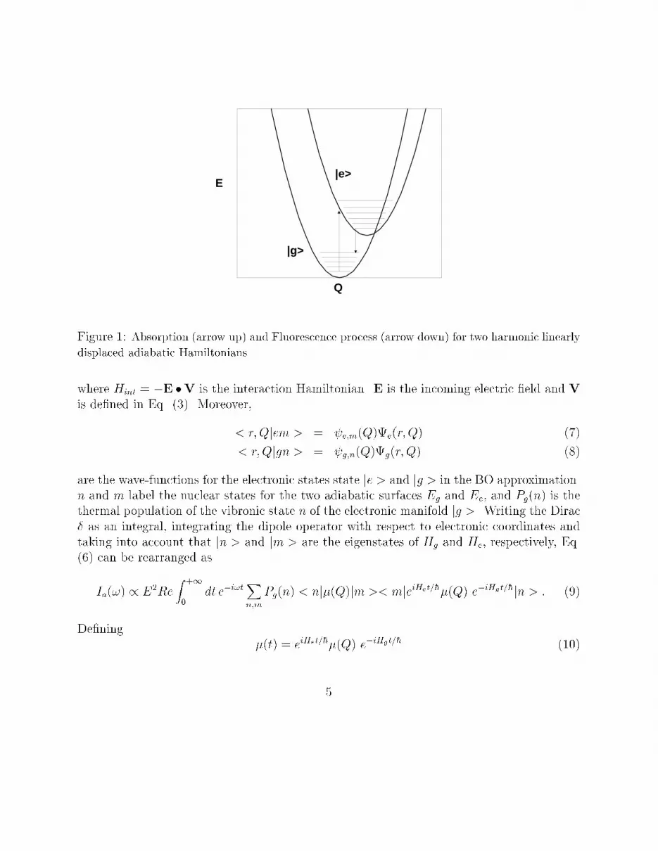
anything but small size molecules2. In order to arrive at the eigenstates Eg(Q) and Ee(Q)for all the Q's sampled in an MD simulation, we �t the two BO surfaces Eg and Ee with asimpli�ed expression based on electro-negativity equalization principle [7] (EE) and partialcharges on the atomic nuclei, using a limited set of ab-initio con�gurations of the solute inthe gas phase (i.e. using H(R; r) only). The �tted surfaces can be tested using con�gurationsof the coordinates R which where not included in the �tting procedure. We then use thesesimpli�ed and computationally inexpensive gas phase BO surfaces plus the electrostaticinteraction with the solvent as a model for the true BO surfaces Eg(Q) and Ee(Q).The present lecture is organized as follows. In section II we shall illustrate a semi-classical approach for the computation of the absorption and uorescence spectra based onthe cumulant expansion of the transition dipole quantum correlation function. In sectionIII we shall illustrate the method for representing the two BO surfaces Eg and Ee usingthe electro-negativity equalization principle. In Section IV, by applying the arguments ofsections II and III to a speci�c example, i.e. the calculation of the absorption and uorescencespectra in formaldehyde, we shall show how this method could represent a computationallyconvenient and powerful tool to evaluate the solvent e�ects on electronic transitions. SectionV contains perspectives and concluding remarks.2 Semi-classical calculation of molecular absorption and uorescence spectraThe treatment developed in this section for the semi-classical expression of the absorptionand uorescence lineshape is heavily based on the work of Mukamel [8, 9, 10].The system corresponds to the adiabatic Hamiltonian (1) and is depicted in Figure 1. Itconsists of two electronic levels jg > and je > coupled to the Q degrees of freedom whichmay include nuclear motions of the solvent and of the solute as well.2.1 AbsorptionIn the framework of linear response, for the absorption cross section Ia(!) of a system initiallyin the electronic state jg >, the Fermi Golden rule holds (prefactor are ignored):Ia(!) / Xn;mPg(n) j he;m j Hint j g; ni j2 �(! � !mn) (6)2The eigenvalues of (4) must be found self-consistently since the electron density � appears explicitly inthe Hamiltonian through the term (5). Note also that a �rst order perturbation approach on V (R;S; r)assumes no polarizability on the solute. 4

|e>

|g>

Q

E

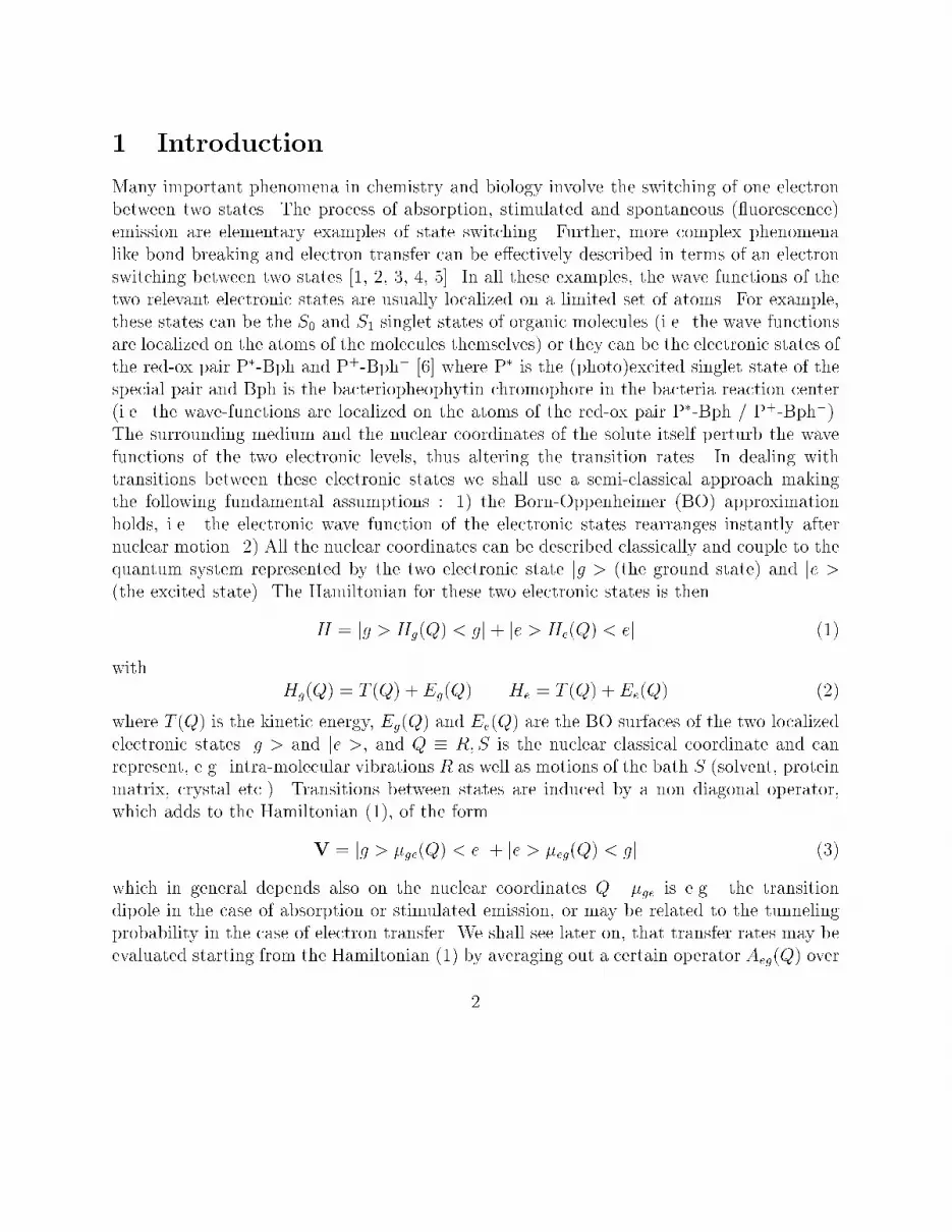
Figure 1: Absorption (arrow up) and Fluorescence process (arrow down) for two harmonic linearlydisplaced adiabatic Hamiltonianswhere Hint = �E �V is the interaction Hamiltonian. E is the incoming electric �eld and Vis de�ned in Eq. (3). Moreover,< r;Qjem > = e;m(Q)e(r; Q) (7)< r;Qjgn > = g;n(Q)g(r; Q) (8)are the wave-functions for the electronic states state je > and jg > in the BO approximation.n and m label the nuclear states for the two adiabatic surfaces Eg and Ee, and Pg(n) is thethermal population of the vibronic state n of the electronic manifold jg >. Writing the Dirac� as an integral, integrating the dipole operator with respect to electronic coordinates andtaking into account that jn > and jm > are the eigenstates of Hg and He, respectively, Eq.(6) can be rearranged asIa(!) / E2Re Z +10 dt e�i!tXn;mPg(n) < nj�(Q)jm >< mjeiHet=�h�(Q) e�iHgt=�hjn > : (9)De�ning �(t) = eiHet=�h�(Q) e�iHgt=�h (10)5

using the fact that Pg(n) =< nj�gjn > with �g � e��Hg=Zg being the density matrix for theHamiltonian Hg and using twice the closure relation one obtainIa(!) / E2Re Z +10 dt e�i!th�(0)�(t)ig (11)where h�(0)�(t)ig = Tr[�g�(0)�(t)]: (12)For the sake simplicity we neglect the Q dependence of �(Q) (Condon approximation [11])and take the transition dipole as a molecular constant. Using Eq. (10) and disregarding thedependence on the incoming �eld E, we may write (11) asIa(!) / Re Z +10 dte�i!theiHet=�h e�iHgt=�hig (13)where heiHet=�h e�iHgt=�hig �Xn Pg(n) < njeiHet=�h e�iHgt=�hjn > (14)The signi�cance of (14) is clear: the correlation function heiHet=�h e�iHgt=�hi may be obtainedstarting at the vibronic state jn >, propagating the wave function for a time t on the Hg andfor a time �t on He. The overlap of the resulting wave-function with the state jn > yieldsthe thermally unweighted contribution to the vibronic state jn > to the correlation function.Due to the evolution on di�erent BO surfaces it is not obvious to devise a semi-classicalanalog of (11). In order to do that, following Mukamel [10], we use the following identitiesdue to Feynmann, valid for any two linear operators AB,e(A+B)t = exp� �Z t0 d� B(�)� eAt (15)e�(A+B)t = e�At exp+ �� Z t0 d� B(�)� (16)where the shorthands exp+; exp� 3 stand for the cumulant expansionsexp� �Z t0 d� B(�)� = 1 + Z t0 d�1B(�1) + Z t0 d�1 Z �10 d�2B(�2)B(�1) + � � � (17)exp+ �� Z t0 d� B(�)� = 1� Z t0 d�1B(�1) + Z t0 d�1 Z �10 d�2B(�1)B(�2) + � � � (18)B(t) = e�AtBeAt: (19)3exp+ and exp� are not conventional exponential since the � -ordered operators in the expansions Eq.(17-18) do not in general commute. 6

We now set in the �rst identity (15)A+B = iHe=�h A = iHg=�h B = i(He �Hg)=�h = iU=�h (20)B(t) = exp(iHgt=�h)Uexp(�iHgt=�h): (21)U(t) is the energy gap operator evaluated on the ground state surface which of course has anobvious classical analog. Substituting Eqs. (20-21) into Eq. (15), the quantum correlationfunction in Eq. (13) can be expressed in terms of the gap only :C(t) = heiHet=�h e�iHgt=�hig = �exp� � i�h Z t0 d� U(�)��g : (22)We now make the ansatz [8]:C(t) = e( i�h)K1(t)+( i�h)2K2(t)+::: (23)where Kn is a n-order term in U . In order to determine K1(t) and K2(t) we equate term byterm the expansions up to the second order in U on the rhs of Eqs.(22) and (23). We obtainto the �rst order K1 = Z t0 d� hU(t)ig =< U >g t (24)where we have used the fact the < U(t) > is time independent for a system at equilibrium,and to the second order K2 = Z t0 d� Z �0 d� 0 hU(� 0)U(�)ig � 12K21 (25)= Z t0 d� Z �0 d� 0 hu(� 0)u(�)ig (26)with u � U �hUig. The �rst order term is merely the average vertical energy gap calculatedon the ground state jg >. The second-order term contains the e�ect of the Q coordinates onthe absorption pro�le and the relevant quantity is the uctuation of the gap U evaluated onthe jg > BO surface. De�ninggg(t) = 1�h2 Z t0 d� Z �0 d� 0 hu(� 0)u(�)ig !eg = < U >g�h (27)inserting these de�nitions into Eqs. (24,26), inserting the resulting equations into Eq. (23)and �nally substituting Eq. (23) into Eq. (13), we arrive at the expression for the absorptionline-shape: Ia(!) / Re Z +10 dt e�i(!t�!eg)�gg(t) (28)7

The practical semi-classical calculation of (28) involve the following steps:I) compute from the MD of the solute and the solvent the classical4 correlation functionhu(�)u(0)ig (in the next section we shall describe a method for computing the gap U(Q(t))),along with its Fourier transform, the spectral densityJc(!) = Z < u(t)u(0) >classicg ei!tdt; (29)II) correct for the detailed balance the spectral density;5.III) arrive at g(t) using the identityg(t) = 1�h2 Z t0 d� Z �0 d� 0 hu(� 0)u(�)ig = Z 1�1 J(!)(�h!)2 (ei!t � i!t� 1)d! (30)and use g(t) to evaluate the spectrum according to (28).It can be shown that expression (28), based on the second order cumulant expansion(24-26) of Eqs. (17,18), is exact, 1) when the modes of the bath are harmonic and linearlydisplaced in going form jg > to je > (i.e. the frequencies of the oscillators are the same forjg > and je > and only the minima are displaced) and 2) when the energy gap distributionfunction P (U(Q)) is Gaussian with the same energy distribution seen from the ground orseen from the excited state. In all other cases (28) is an approximation.The second order cumulant expansion is better suited for medium size highly vibrationallyexcited molecules than for simple diatomic or triatomic molecules [9]. Conditions 2) are infact usually met in large molecules where there exist many vibrational modes and wherethe distribution of these modes changes slightly in going from the ground to the excitedstate. Also, for large molecules the use of the classical correlation function hu(�)u(0)i forthe calculation of the spectral density J(!) is more justi�ed since the highly populatedlow frequency modes, which contribute most to the absorption lineshape, behave essentiallyclassically.4The solute classical dynamics and its interaction with the solvent is done with a parameterization of thepotential relative to the ground state surface5This step may be not necessary at high temperature. However the classical spectral density exhibitsthe symmetry Jc(�!) = Jc(!) while in fact the true quantum spectral density satis�es the detailed balancecondition Jq(�!) = e���h!Jq(!)). To correct for the detailed balance condition, several procedures havebeen proposed [12, 13, 14]8

2.2 FluorescenceWe consider now, the emission6 of the system, initially at the equilibrium in the excited state.The starting point is again the expression (6) where Pg(n) is simply replaced by Pe(m) andthe bra < mj and and ket jn > are exchanged. Like we did for the absorption line shape, wewrite the transition rate in terms of a correlation function which has to be computed thistime on the He BO surface. Using the second Feynmann identity (16) withA+B = iHg=�h A = iHe=�h B = i(Hg �He)=�h = iU=�h (31)B(t) = exp(iHet=�h)Uexp(�iHet=�h) (32)and doing exactly the same steps as described in the previous subsection we arrive at theexpression for the uorescence line-shapeIf(!) / Re Z +10 dt e�i(!�!0eg)t�ge(�t) (33)where !0eg = hUie =�h and ge(t) is identical to (27) except that this time the averages of theenergy gap and of its uctuation are taken over the excited state BO surface. This fact issomewhat inconvenient since one has normally a classical parameterization of only one of thetwo surfaces Eg and Ee, usually the ground state. To use Eq. (33) one is forced do anothersimulation using an excited state parameterization for generating the solute con�gurationsR.7To avoid doing the excited state parameterization and to avoid sampling the Q coordi-nates on this BO surface, we want to �nd an expression which allows us to compute the uorescence band pro�le taking the averages on the ground state surface [15]. To this end,we start from the expressionC(t) = Tr he�iHgt=�heiHet=�he��Hei =Ze (34)which is the correlation function of interest in our case. We use following identities,eiHet=�h = eiHgt=�h exp+ � i�h Z t0 d� U(��)�e��He = exp� "� Z �0 d�U(i��h)# e��Hg (35)6With the term \ uorescence" we indicate actually the relaxed uorescence, tacitally assuming that thenuclear degrees of freedom relaxes very rapidly compared to the radiative lifetime of the je > electronic state.7For example the excited state parameterization may have the same frequency distribution of the vibra-tional modes given by the ground state parameterization but may have a di�erent dipole moment whichinteracts di�erently with the classical solvent 9

where U = He � Hg, U(t) = eiHgt=�hUe�iHgt=�h. In the second equation we have simply used(16) with (A+B) = i(i��hHe)=�h and A = i(i��hHg)=�h. Substituting (36) into (34) one gets:C(t) = ZgZe *exp+ � i�h Z t0 U(��)d�� exp� "� Z �0 U(i��h)d�#+g (36)where the averages are taken on the g BO surface. As usual, we make the ansatz (23) onthe correlation function (37) and equate term by term the expansions of the rhs of Eq. (37)based on the identities Eqs. (36) and the Taylor expansion of Eq. (23). We give here the�nal result which is C(t) = ZgZe e i�h hUigt��hUig�gg(t)+fg(t)+gg(i�h�) (37)where gg(t) = 1�h2 Z t0 d� Z �0 d� 0 hu(� 0)u(�)ig (38)fg(t) = � i�h Z t0 d� Z �0 d� hu(��)u(i��h)ig (39)and gg(i�h�) = Z �0 d�1 Z �10 d�2 hu(i�2�h)u(i�1�h)ig (40)The �nal expression for the uorescence line-shape is :I 0f (!) / A0Re Z +10 dt e�i(!t�!eg)te�gg(t)+fg(t) (41)where !eg = hUig =�h and A0 = ZeZg e��hUig+g(i�h�). The factor A0 is just a multiplicativeconstant which does not alter the band-shape. Again, for the practical computation of the uorescence intensity (42), we must �rst evaluate the spectral density J(!) (Eq.(29)). Simpleexpressions relates then the spectral density to the functions gg(t); fg(t); gg(i�h�).3 Parameterization of the BO surfacesIn this section we describe a simple semi-empirical method to evaluate the energies Eg andEe based on a simpli�ed density functional approach [16, 17, 18]. The basic variationalprinciple in density functional theory reads� �E[�]� ��Z �(r)�N�� = 0 (42)10

The ground state energy E[�] is a unique functional of the electron density �. Eq. (43)expresses the fact that, to arrive at the true ground state energy, the energy must be mini-mized with respect to �, subject to the normalization condition that � must integrate to N,the total number of electron in the system. Here � is an undetermined Lagrange multiplierand equals to the functional derivative of the energy with respect to the density.� = �E[�]�� (43)The quantity � is the chemical potential. Eq. (44) is valid for any system. For molecules atequilibrium, in particular, Eq. (44) states that � is a constant everywhere on the molecule[19, 20, 21]. Eq. (44) is the physical basis upon which the scheme of electro-negativityequalization discussed hereafter is based.3.1 Electro-negativity equalization principleWe now write the energy of an atom as function of the number of electron and we expandup to the second order around N0 = Z, where Z is the nuclear chargeE(N) = E(N0) + @E@N !0 (N �N0) + 12 @2E@N2!0 (N �N0)2 (44)E(q) = E(0) + @E@q !0 q + 12 @2E@q2 !0 q2: (45)In the second equation we have de�ned the partial charge on the atom as q = �e(N � Z)with e being the charge of the electron. Let us see the relationship between @E=@q and@2E=@q2 with the familiar concepts of electro-negativity, ionization potential and electrona�nity. If we subtract and add one electron to the atom, by virtue of Eq. (46) we have thatI = E(+1)� E0 = @E@q !0 + 12 @2E@q2 !0 (46)A = E0 � E(�1) = @E@q !0 � 12 @2E@q2 !0 (47)where I and A are the ionization potential and the electron a�nity. Hence@E@q = I + A2 = �@2E@q2 = I � A = � (48)11

� is a positive quantity de�ned as the electro-negativity of the atom and is the negative ofthe chemical potential (@E=@q = �@E=@N = �� ). As to the electro-negativity �, equation(49) agrees with the familiar concept that strongly electro-negative atoms \like" electrons:such atoms gain energy by acquiring one electron (A high) and spend energy by loosing one(I high). The quantity � is termed hardness [22, 23] of the atom. It may be viewed as theresistance to do the dismutation relation 2 _A! A� + A+. \Hard" atoms are happy as theyare: neither they like to acquire electrons nor they get pleasure in loosing them. Due to theconvexity of the ground state energy with respect to the density [24], it can be shown thatthe hardness is also a positive quantity [19, 25]. Let us now consider a diatomic heteronuclearmolecule AB in the gas phase. The chemical potential (or electro-negativity) equalizationprinciple (44) requires that � is equal all over the molecule. The molecular energy isEmol = EA + EB= E0AB + �A0qA + �B0qB + 12(�A0q2A + �B0q2B) + f(R)qAqBR (49)where E0AB = EA + EB is the energy in an ideal molecular reference state with no chargeseparation [16, 26] and �A0 = @E@qA!0 �B0 = @E@qB!0 (50)�A = @2E@q2A !0 �B = @2E@q2B !0 (51)are the electro-negativities and hardnesses in this ideal state. The last term in Eq. (50)represents the interaction between the two charge densities qA and qB. The function f(R) isa screening factor [27, 17] that goes to 1 as the inter-nuclear distance R goes to in�nity, suchthat the charge-charge interaction tends to the Coulomb potential. We take for example afunction of the form f(R) = �1� e�aRs� (52)where a and s are adjustable parameters. Charge transfer occurs from regions of the moleculewhere the electro-negativity is high to regions where the electro-negativity is low so as toequalize �, i.e. the chemical potential, everywhere on the molecule. To �nd the equilibriumcharges we therefore need solve the linear system@E@qA = �A = �B = @E@qBqmol = qA + qB = 0: (53)12

0.5 1.0 1.5 2.0 2.5-1.5

-1.0

-0.5

0.0

0.5

1.0

e

eV

R

E(R)

q(R)

(Angs)

χ = 3η = 32

a=2s=4

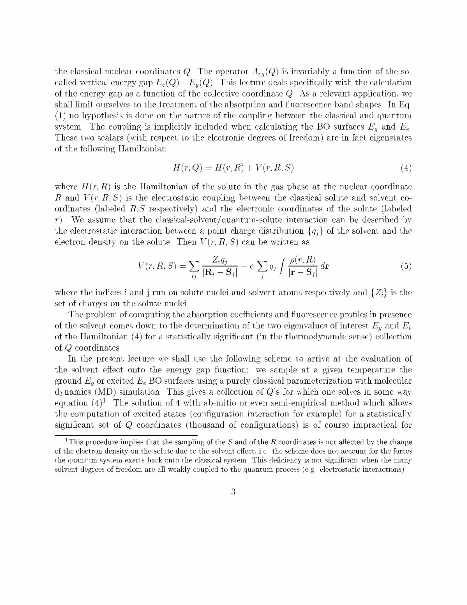
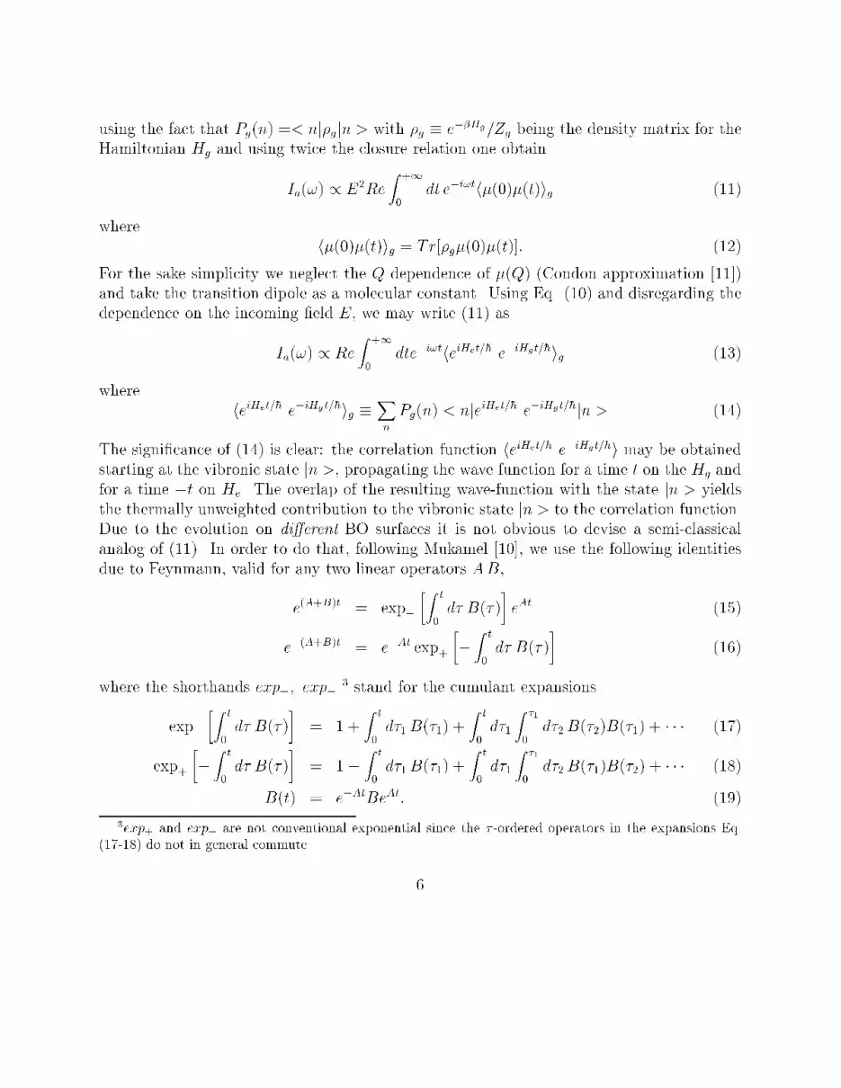
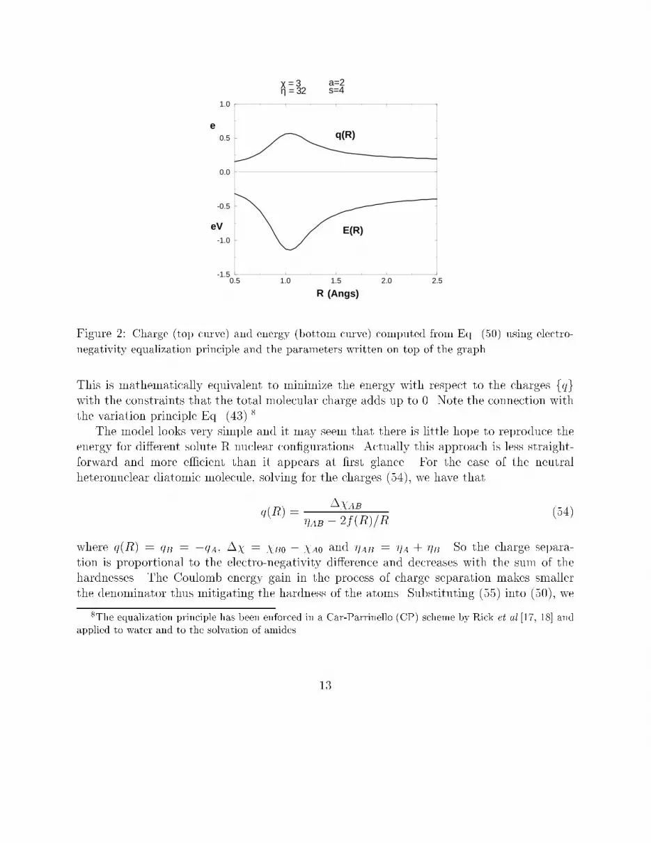
Figure 2: Charge (top curve) and energy (bottom curve) computed from Eq. (50) using electro-negativity equalization principle and the parameters written on top of the graph.This is mathematically equivalent to minimize the energy with respect to the charges fqgwith the constraints that the total molecular charge adds up to 0. Note the connection withthe variation principle Eq. (43).8The model looks very simple and it may seem that there is little hope to reproduce theenergy for di�erent solute R nuclear con�gurations. Actually this approach is less straight-forward and more e�cient than it appears at �rst glance. For the case of the neutralheteronuclear diatomic molecule, solving for the charges (54), we have thatq(R) = ��AB�AB � 2f(R)=R (54)where q(R) = qB = �qA, �� = �B0 � �A0 and �AB = �A + �B. So the charge separa-tion is proportional to the electro-negativity di�erence and decreases with the sum of thehardnesses. The Coulomb energy gain in the process of charge separation makes smallerthe denominator thus mitigating the hardness of the atoms. Substituting (55) into (50), we8The equalization principle has been enforced in a Car-Parrinello (CP) scheme by Rick et al.[17, 18] andapplied to water and to the solvation of amides. 13

obtain the molecular energyER = E0AB � q(R)��AB + 12�AB � f(R)R ! q(R)2 (55)In Figure 2 we plot the function E(R) (in eV) (E0AB is just an additive constant and istaken to be zero) and the charge q (in electron) as a function of R for a diatomic with��AB = 4:0 eV , �AB = 32:0 eV , a = 2:0 �A�1 and s = 4. The �t of E(R) and of the dipoleis not too bad for the region around the minimum for the ground singlet state of HF.3.2 Fitting the BO surfaces in polyatomic moleculesThe extension of Eq. (50) to the case polyatomic molecules is trivial: we have thatEmol = E0 + MXi=1 ��i0qi + 12�iq2i � + 12 MXi 6=j f(Rij)qiqjRij (56)whereM is the number of atoms in the molecule.9 For the parameters a and s in Eq. (53) weuse the sum rule aij = ai + aj and sij = si + sj where ai and si are atomic parameters. Thecharges qi on the molecules are found by imposing theM�1 conditions for electro-negativityequalization �1 = �2 = ::: = �M and the additional condition of neutrality. This leads tothe following linear system0BBBBBB@ 0�10 � �20�10 � �30::�10 � �M01CCCCCCA = 0BBBBBB@ 1 1 :: 1F21 F22 :: F2M:: :: :: :::: :: :: ::FM1 FM2 :: FMM

1CCCCCCA0BBBBBB@ q1q2::::qM1CCCCCCA (57)where the matrix element Fij is given byFij = Gij �G1j i 6= 1 (58)Gij = �ij�i + (1� �ij)f(Rij; ais; sij)Rij (59)9M does not necessarily coincide with the total number of nuclei in the molecule. M could be wellrestricted to the atoms whose AO0s contribute most to the HOMO and LUMO orbitals: e.g. in bacteri-ochlorophyll the propionic side chains could have �xed charges and the EE may be applied only to the atomsof the planar ring. 14

We use Eq. (57) to �t the E(R) BO surface of both the ground and the excited states10with respect to the parameters �i, �i, ai and si. The quantity E0 in (57) is also a variationalparameter. In general there are four �, �, a and s parameters for each kind of chemicallyinequivalent atom. For example in complex organic molecules, one may �nd convenient todistinguish between sp2 or sp3 carbons. From now on we shall indicate with the collectivesymbol p � �i; �i; ai; si with i = 1; ::mt, the ensemble of variational parameters in Eq. (57).The �t is done as follow. Suppose we are interested in the S0 and S1 singlet state of aneutral molecule. We solve the gas phase Hamiltonian H(R; r) in Eq. (4) using an ab initiomethod for a few con�gurations. The selected con�guration are sampled with MD at thewanted temperature using a purely classical parameterization of the ground state only. Letthis reduced set be indicated with R = R1; :::Rconf . Further, we indicate withE(g)(Rk); d(g)(Rk) (60)E(e)(Rk); d(e)(Rk) (61)the ab initio energies and dipoles of the ground and excited singlet states S0 and S1 forthe reduced set of gas phase con�gurations R. The sampling using MD with a correctparameterization on the ground state assures that the di�erence of bond lengths and bendangles from their equilibrium values are compatible with the amplitude of these motions atthe given temperature. This is done so as to select the con�gurations R in the range wherethey are actually needed and not in region of R which are not accessible. For the reducedset fRg we �nd the parameter vector p which best �t the ab initio energies and the dipolesof the ground state for the restricted set fRg; i.e. we minimize the functionF = nconfXk (E(Rk;p)� E(g)(Rk))2 +WX� (d�(Rk;p)� d(g)� (Rk))2 (62)where W is a weighting factor to be adjusted11. For a given set of trial parameters p thenconf con�gurational energies E(Rk;p) and dipoles d(Rk;p) are computed by solving nconftimes the system (58) and then using the resulting charges qik to calculate the dipoled(RK) =Xi qikrik; (63)where rik is the position vector of the i-the atom for the k-th con�guration Rk, and theenergy using (57).10Eq. (43) is strictly valid only for the ground state. Hence for the excited state BO surface (57) is just a�tting function and the connection with the variation principle (43) is no longer valid.11One can also �t the polarizability of the molecule which can be easily computed with the EE basedmodels [28, 29, 17] 15

We refer to the optimal parameters which minimize F (Eq. (63)) as pg to indicate thatthese parameters reproduce the energies and the dipoles of the ground state.Since we are interested in the vertical energy gap starting from the ground state forboth absorption and uorescence spectra (See Eqs. (28,42)), we use the same set R to �tthe excited state surface. We must hence minimize the function (63) where Eg(Rk) andd(g)(Rk) are replaced by the excited state Ee(Rk) and d(e)(Rk) values. In this fashion wehave determined the \Hamiltonians" for the two surfaces Eg and Ee in the gas-phase andnear the minimum of the Eg surface (see Figure 3). To �nd the energy Eg and Ee andthe corresponding charge distributions for any con�guration R, it su�ces to solve twice thelinear system (58), once with the parameters pg - and we �nd Eg - and the second time withthe parameter pe - and we �nd Ee. To �nd the energies Eg;e(Q) in presence of the solvent,on the basis of Eq. (4), we postulate that this energy is given byEg(Q) = E(pg; q1:::qM) +Xik qiq(0)kjRi � Skj = E(pg; q1:::qM) +Xi qiVi(Q)Ee(Q) = E(pe; q1:::qM) +Xik qiq(0)kjRi � Skj = E(pe; q1:::qM ) +Xi qiVi(Q): (64)Here the index k runs over the solvent atomic charges q(0)k and we have de�ned the solventelectrostatic potential at atom i asVi(Q) =Xk q(0)kjRi � Skj : (65)The additional term to the gas phase energy, i.e the Coulomb energy between the �xedcharges on the solvent q0k and the charges on the solute qi, plays the role of the solventperturbation Hamiltonian V (r; R; S) (Eqs. (4-5)). It depends on the solvent and solutenuclear coordinates R; S and on the \electronic" coordinates of the solute q � r. For a givensystem con�guration Q, in order to get the energies Eg(Q) and Ee(Q), we use the gas phaseparameters pe and pg and we solve the linear systems obtained by minimizing the energies(65) with respect to the solute atomic charges qi0BBBBBB@ 0�10 � �20 + V1(Q)� V2(Q)�10 � �30 + V1(Q)� V3(Q)::�10 � �M0 + V1(Q)� VM(Q)1CCCCCCA = 0BBBBBB@ 1 1 :: 1F21 F22 :: F2M:: :: :::: :: ::FM1 FM2 :: FMM

1CCCCCCA0BBBBBB@ q1q2::::qM1CCCCCCA (66)16

∆Ε

∆Ε

e

g

R

|e>

|g>

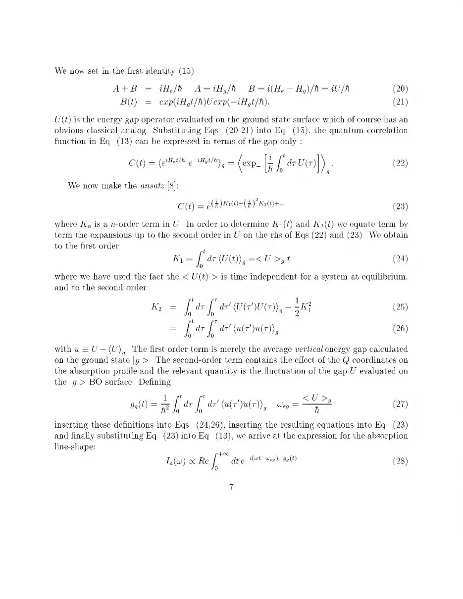
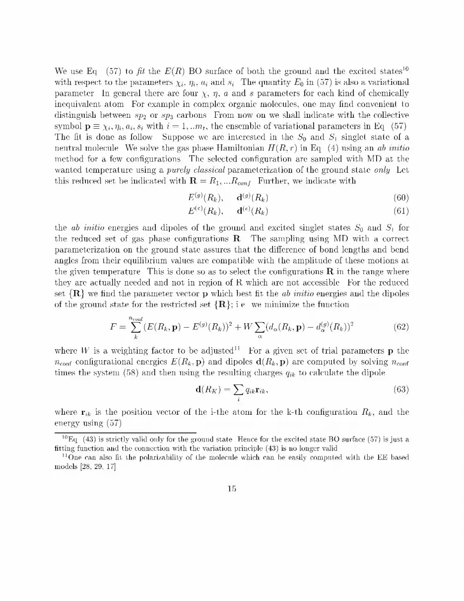
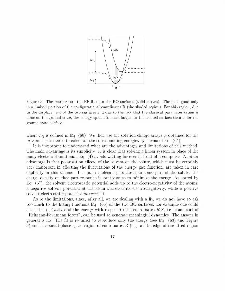
Figure 3: The markers are the EE �t onto the BO surfaces (solid curves). The �t is good onlyin a limited portion of the con�gurational coordinates R (the shaded region). For this region, dueto the displacement of the two surfaces and due to the fact that the classical parameterization isdone on the ground state, the energy spread is much larger for the excited surface than is for theground state surfacewhere Fij is de�ned in Eq. (60). We then use the solution charge arrays qi obtained for thejg > and je > states to calculate the corresponding energies by means of Eq. (65).It is important to understand what are the advantages and limitations of this method.The main advantage is its simplicity. It is clear that solving a linear system in place of themany-electron Hamiltonian Eq. (4) avoids waiting for ever in front of a computer. Anotheradvantage is that polarization e�ects of the solvent on the solute, which must be certainlyvery important in a�ecting the uctuations of the energy gap function, are taken in careexplicitly in this scheme. If a polar molecule gets closer to some part of the solute, thecharge density on that part responds instantly so as to minimize the energy. As stated byEq. (67), the solvent electrostatic potential adds up to the electro-negativity of the atoms:a negative solvent potential at the atom decreases its electro-negativity, while a positivesolvent electrostatic potential increases it.As to the limitations, since, after all, we are dealing with a �t, we do not have to asktoo much to the �tting functions Eq. (65) of the two BO surfaces: for example one couldask if the derivatives of the energy with respect to the coordinates R,S, i.e. some sort of\Helmann-Feynmann forces", can be used to generate meaningful dynamics. The answer ingeneral is no. The �t is required to reproduce only the energy (see Eq. (63) and Figure3) and in a small phase space region of coordinates R (e.g. at the edge of the �tted region17

-442.96 -442.94 -442.92 -442.90-442.96

-442.94

-442.92

-442.90 |g>

eV

-440.20 -440.15 -440.10-440.20

-440.15

-440.10

eV

eV

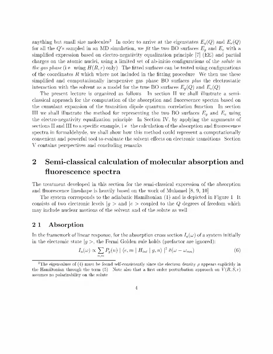
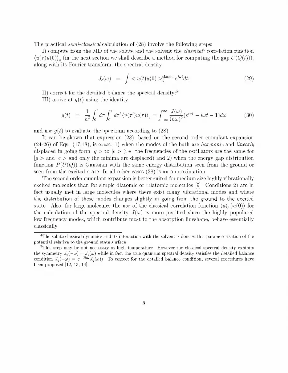
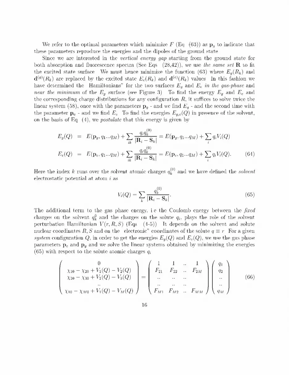
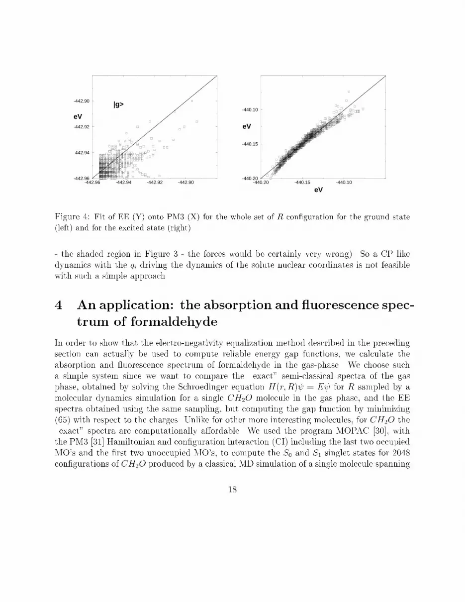
Figure 4: Fit of EE (Y) onto PM3 (X) for the whole set of R con�guration for the ground state(left) and for the excited state (right)- the shaded region in Figure 3 - the forces would be certainly very wrong). So a CP likedynamics with the qi driving the dynamics of the solute nuclear coordinates is not feasiblewith such a simple approach.4 An application: the absorption and uorescence spec-trum of formaldehydeIn order to show that the electro-negativity equalization method described in the precedingsection can actually be used to compute reliable energy gap functions, we calculate theabsorption and uorescence spectrum of formaldehyde in the gas-phase. We choose sucha simple system since we want to compare the \exact" semi-classical spectra of the gasphase, obtained by solving the Schroedinger equation H(r; R) = E for R sampled by amolecular dynamics simulation for a single CH2O molecule in the gas phase, and the EEspectra obtained using the same sampling, but computing the gap function by minimizing(65) with respect to the charges. Unlike for other more interesting molecules, for CH2O the\exact" spectra are computationally a�ordable. We used the program MOPAC [30], withthe PM3 [31] Hamiltonian and con�guration interaction (CI) including the last two occupiedMO's and the �rst two unoccupied MO's, to compute the S0 and S1 singlet states for 2048con�gurations of CH2O produced by a classical MD simulation of a single molecule spanning18

8 ps at 400 K (due care has been taken to equalize the kinetic energy on each intra-moleculardegree of freedom). For the classical parameterization of formaldehyde we used the AMBER[32, 33] force �eld parameters for the internal vibrations. It can be argued that we couldhave used a true ab-initio method in place of the semi-empirical PM3 parameterization. ThePM3 method for small organic molecules is cheap and gives result comparable to other muchmore expensive ab-initio methodology.For formaldehyde, using CI with four orbitals in the open shell manifold, MOPAC predictsan average vertical energy gap of about 2:7 eV to be compared to the experimental valueof 3:1 eV [34]. The dipole predicted by MOPAC at the optimum geometry in the groundstate is 2:0 D (the experimental value is 2:3 D[35]) and 1:8 D in the excited state (theexperimental value is 1:6 D[36]). However, provided that the S0 and S1 surfaces near theminimum of S0 are reasonably realistic, for our purposes PM3, B3-LYP, MP2 HF-CI etc. areall alike. Here, we are not truly interested in the spectra of CH2O but we just want to showthat the �tting procedure described in the previous section allows to compute uorescenceand absorption spectra which closely resemble to those computed using an ab initio or goodsemi-empirical method.Table 1: Fitted parameters for the S0 electronic ground state in CH2O; see text for themeaning of the symbolstype � (eV=e) � (eV=e2) 1=a (�A) sO 7.6460 16.4203 0.6098 4.9024C 5.1031 13.0251 0.8461 3.5193H 5.0857 17.4085 0.8311 3.3869E0 (eV ) -442.4126Table 2: Fitted parameters for the �rst singlet excited state (S1) in CH2O; see text for themeaning of the symbolstype � (eV=e) � (eV=e2) 1=a (�A) sO 12.4297 21.4972 2.1911 5.2399C 7.1314 10.1755 1.2939 4.4913H 6.5955 24.4619 0.0005 1.7135E0 (eV ) -438.979119

0.00

EE

PM3

3000 cm -1

0-0 transition

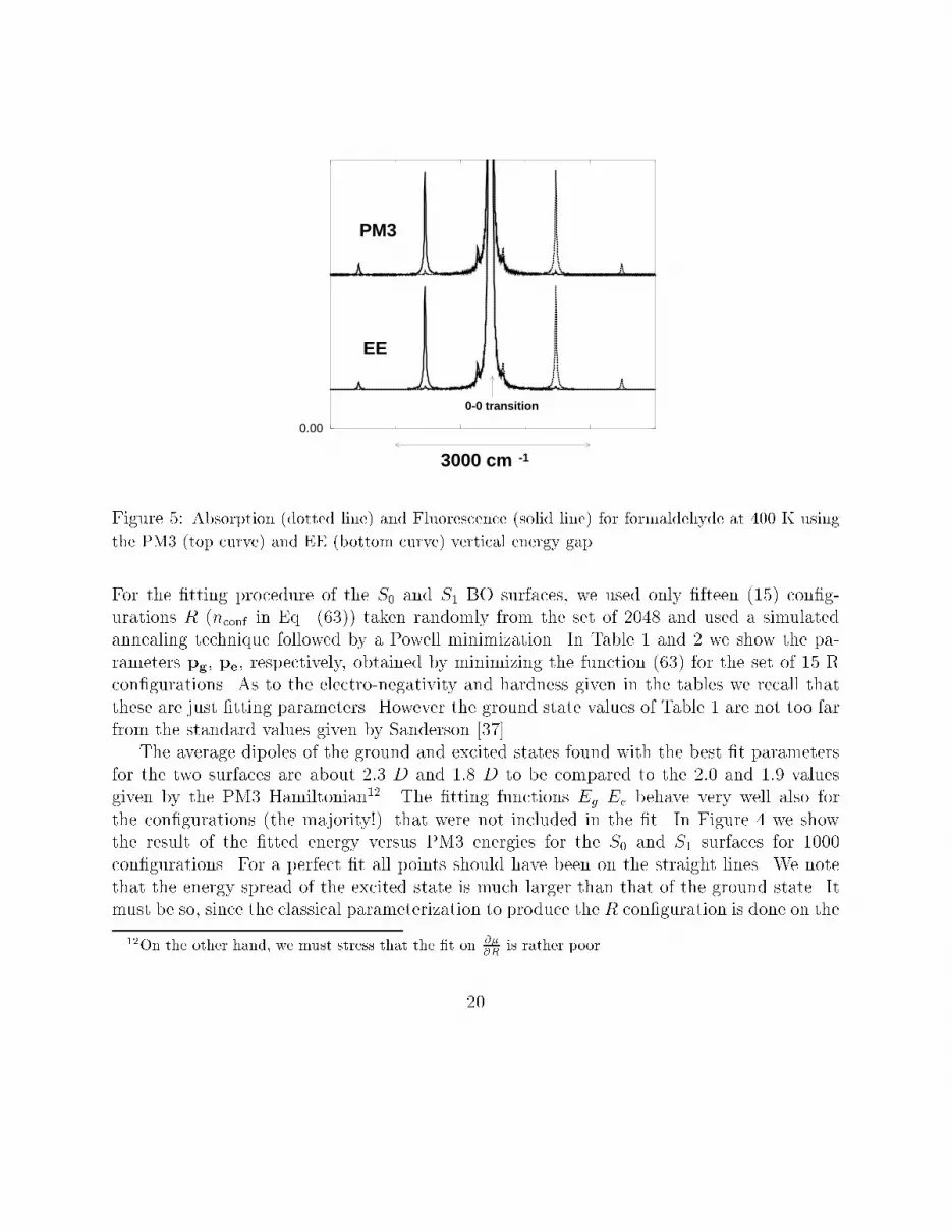
Figure 5: Absorption (dotted line) and Fluorescence (solid line) for formaldehyde at 400 K usingthe PM3 (top curve) and EE (bottom curve) vertical energy gapFor the �tting procedure of the S0 and S1 BO surfaces, we used only �fteen (15) con�g-urations R (nconf in Eq. (63)) taken randomly from the set of 2048 and used a simulatedannealing technique followed by a Powell minimization. In Table 1 and 2 we show the pa-rameters pg, pe, respectively, obtained by minimizing the function (63) for the set of 15 Rcon�gurations. As to the electro-negativity and hardness given in the tables we recall thatthese are just �tting parameters. However the ground state values of Table 1 are not too farfrom the standard values given by Sanderson [37].The average dipoles of the ground and excited states found with the best �t parametersfor the two surfaces are about 2:3 D and 1:8 D to be compared to the 2:0 and 1:9 valuesgiven by the PM3 Hamiltonian12. The �tting functions Eg Ee behave very well also forthe con�gurations (the majority!) that were not included in the �t. In Figure 4 we showthe result of the �tted energy versus PM3 energies for the S0 and S1 surfaces for 1000con�gurations. For a perfect �t all points should have been on the straight lines. We notethat the energy spread of the excited state is much larger than that of the ground state. Itmust be so, since the classical parameterization to produce the R con�guration is done on the12On the other hand, we must stress that the �t on @�@R is rather poor20

ground state, and hence around the minimum of the surface Eg(R) but in region of steepervariation for the displaced surface Ee (see Figure 3). It is important to understand that the�t is good only in the sampled region at the selected temperature (see Figures 3,4). At leastfor the purposes of computing the absorption and uorescence spectra, for relatively rigidmolecule and in the hypothesis that the transition are vertical (i.e. the Born-Oppheneimerapproximation holds) this is actually the only region where we want the �t to be good. InFigure 5 the EE absorption and uorescence spectra are compared to the PM3 counterpart(the \exact" spectra). The spectra have been calculated using the semi-classical expressions(28) and (33) for absorption and uorescence, respectively. The �tted EE and exact PM3spectra are essentially identical.5 Conclusions and perspectivesWe have shown that EE based parameterizations of BO surfaces are able, in principle, toreproduce satisfactorily the energy gap function obtained with ab initio methods. Thisgap function could be then used to compute, starting from the con�gurations obtained byclassical MD, the absorption and uorescence spectra of medium and large size moleculeusing the semi-classical approach based on the second order cumulant expansion of thetransition dipole quantum correlation function. Unfortunately, using the simple EE functionwith the screening factor (53) and the second order expansion (46), one does not have a �tof the dipole moment (and of the polarizability) of the same quality of that obtained for theenergy. This is especially true when the size of the molecule grows. For large molecules withhighly delocalized HOMO and LUMO, the S0 and S1 minima are only slightly displaced andthe di�erence between the two electronic states is mainly in the electron density (i.e. in thecharge distribution). We have veri�ed that adding a term depending on q3 to the expansion(46) improves notably the �t of both dipole and energy. On the other hand, using a thirdorder expansion of the energy, when equalizing the electro-negativities, one ends up with anon linear system which has to be solved iteratively.The EE method could be also improved and extended to produce the intra-moleculardynamics of the solute coordinates R on the jg > surface (e.g. using the adiabatic bondcharge model [38, 29]). The classical parameterization of the jg > surface would then be nolonger needed since the R coordinates could be sampled using the EE parameterization itself.An extended system molecular dynamics method for EE has been already implemented.[17,18].Finally, a last comment on the solvent model: in Eqs. (4-5) we have assumed that thesolvent electron density may be described through a unpolarizable point charge distribution.21

However, the EE scheme could be extended to the solvent ground state electron density aswell. This would make solvent molecules polarizable as they actually are. As to absorptionand uorescence spectra, it has been shown that solvent polarization has a little e�ect onthe band-shapes but may a�ect the solvent reorganization energy and stokes shifts [39].References[1] R. A. Marcus. J. Am. Chem. Soc., 24:966, 1956.[2] R. A. Marcus. J. Am. Chem. Soc., 24:979, 1956.[3] J. S. Bader, R. A. Kuharski, and D. Chandler. J. Chem. Phys., 93:230, 1990.[4] K. Schulten and M. Tesch. Chem. Phys., 158:421, 1991.[5] J. N. Gehlen, D. Chandler, H. J. Kim, and J. T. Hynes. J. Phys. Chem, 96:1748, 1992.[6] M. Marchi, J.N. Gehlen, D. Chandler, and M. Newton. J. Am. Chem. Soc., 115:4178,1993.[7] R. T. Sanderson. Science, 114:670, 1951.[8] S. Mukamel. J. Chem. Phys., 77:173, 1982.[9] S. Mukamel. J. Phys. Chem, 89:1077, 1985.[10] S. Mukamel. Non Linear Optical Spectroscopy. Oxford University Press, 200 MadisonAve, New York NY 10016, 1995.[11] G. Herzberg. Spectra of Diatomic Molecules. Van Nostrand, New York, 1950.[12] P. Egelste�. Adv. Phys., 11:203, 1962.[13] B. J. Berne, J. Jortner, and R. G. Gordon. J. Chem. Phys., 47:1600, 1967.[14] J. Borysow, M. Moraldi, and L. Frommhold. Mol. Phys., 56:913, 1985.[15] M. Souaille and M. Marchi. J. Am. Chem. Soc., 119:3948, 1997.[16] W. J. Mortier, S. K. Ghosh, and S. Shankar. J. Am. Chem. Soc., 108:4315, 1986.22

[17] S. W. Rick, S. J. Stuart, and B. J. Berne. J. Chem. Phys., 101:6141, 1994.[18] S. W. Rick and B. J. Berne. J. Am. Chem. Soc., 118:672, 1996.[19] R. G. Parr, R. A. Donnely, M. Levy, and W. E. Palke. J. Chem. Phys., 68:3801, 1978.[20] N. H. March. J. Chem. Phys., 86:2262, 1982.[21] P. Politzer and H. Weinstein. J. Chem. Phys., 71:4218, 1979.[22] L. Komorowski. Chem. Phys. Letters, 134:536, 1987.[23] R. G. Parr and R. G. Pearson. J. Am. Chem. Soc., 105:7512, 1983.[24] R. G. Parr. Density Functional Theory of Atoms and Molecules. Oxford UniversityPress, 200 Madison Ave, New York NY 10016, 1989.[25] R. A. Donnely and R. G. Parr. J. Chem. Phys., 69:443, 1978.[26] K. T. No, J. A. Grant, and H. A. Scheraga. J. Phys. Chem, 94:4732, 1990.[27] A. K. Rapp�e and W. A. Goddard. J. Phys. Chem, 95:3358, 1991.[28] S. Go, H. Bilz, and M. Cardona. Phys. Rev. Letters, 34:580, 1975.[29] S. Sanguinetti, G. Benedek, M. Righettti, and G. Onida. Phys. Rev. B, 50:6743, 1994.[30] J. J. P. Stewart. MOPAC Manual - Seventh Edition. QCPE, Bloomington Indiana,(1993).[31] J. J. P. Stewart. J. Comp. Chem, 20:221, 1989.[32] S. J. Wiener, P. A. Kollmann, D. T. Nguyen, and D. A. Case. J. Comput. Chem., 7:230,1986.[33] W. D. Cornell, P. Cieplak, C. I. Bavly, I. R. Gould, K. M. Merz Jr., D. M. Ferguson,D. C. Spellmeyer, T. Fox, J. W. Caldwell, and P. Kollmann. J. Am. Chem. Soc.,117:5179, 1995.[34] G. Herzberg. Molecular Spectra and Molecular Structure: III. Electronic Spectra ndElectronic Structure of Polyatomic Molecules. Van Nostrand, New York, 1966.[35] K. Kondo and T. Oka. J. Phys. Soc. Jpn., 15:307, 1960.23

[36] V. T. Jones and J. B. Coon. J. Mol. Spectroscopy, 31:137, 1969.[37] R. T. Sanderson. Chemical Bonds and Bond energy. Academic Press, New York, 1976.[38] W. Weber. Phys. Rev. B, 15:4789, 1977.[39] J. S. Bader and B. J. Berne. J. Chem. Phys., 104:1293, 1996.

24