Blind Audio Source Separation

��

��

��

��

centre for digital music

Blind Audio Source SeparationEMMANUEL VINCENT, MARIA G. JAFARI, SAMER A. ABDALLAH,

MARK D. PLUMBLEY AND MIKE E. DAVIES

Technical Report C4DM-TR-05-0124 november 2005

Blind Audio Source Separation

Emmanuel Vincent, Maria G. Jafari, Samer A. Abdallah, Mark D. Plumbley and Mike E. Davies

Centre for Digital MusicQueen Mary, University of London

Mile End Road – London E1 4NS – United [email protected]

Abstract: Most audio signals are mixtures of several audio sources which are active simultaneously. Forexample, live debates are mixtures of several speakers, music CDs are mixtures of musical instrumentsand singers, and movie soundtracks are mixtures of speech, music and natural sounds. Blind Audio SourceSeparation (BASS) is the problem of recovering each source signal from a given mixture signal. This reportprovides a tutorial review of established and recent BASS methods as applied to the separation of real-istic audio mixtures, focusing on situations where large microphone arrays or other unusual microphonearrangements are not available. Our first goal is to show that a large range of assumptions can be made toseparate a given mixture signal. Our second goal is to emphasize the importance of audio-specific issuesin the design of BASS algorithms. Thus we consider the BASS problem in its full generality and we pointout the modeling assumptions and the limitations of each class of algorithms. For the sake of clarity, wedescribe approaches relating to different historical viewpoints within a general statistical framework. Wedo not discuss implementation details nor other problems related to BASS such as dereverberation andremixing.

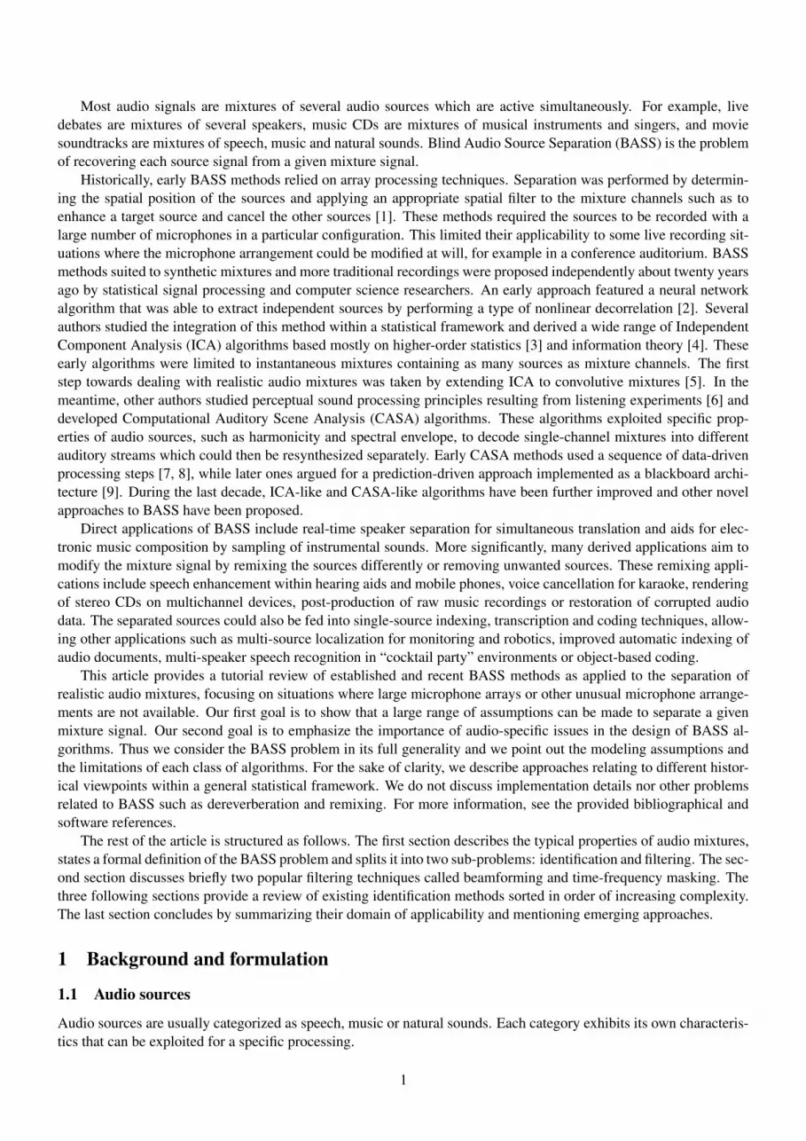
Keywords: source separation, music, speech, recording, CD, beamforming, time-frequency masking, in-dependent component analysis, DUET, factorial hidden Markov model, nonnegative matrix factorization,computational auditory scene analysis.

Most audio signals are mixtures of several audio sources which are active simultaneously. For example, livedebates are mixtures of several speakers, music CDs are mixtures of musical instruments and singers, and moviesoundtracks are mixtures of speech, music and natural sounds. Blind Audio Source Separation (BASS) is the problemof recovering each source signal from a given mixture signal.

Historically, early BASS methods relied on array processing techniques. Separation was performed by determin-ing the spatial position of the sources and applying an appropriate spatial filter to the mixture channels such as toenhance a target source and cancel the other sources [1]. These methods required the sources to be recorded with alarge number of microphones in a particular configuration. This limited their applicability to some live recording sit-uations where the microphone arrangement could be modified at will, for example in a conference auditorium. BASSmethods suited to synthetic mixtures and more traditional recordings were proposed independently about twenty yearsago by statistical signal processing and computer science researchers. An early approach featured a neural networkalgorithm that was able to extract independent sources by performing a type of nonlinear decorrelation [2]. Severalauthors studied the integration of this method within a statistical framework and derived a wide range of IndependentComponent Analysis (ICA) algorithms based mostly on higher-order statistics [3] and information theory [4]. Theseearly algorithms were limited to instantaneous mixtures containing as many sources as mixture channels. The firststep towards dealing with realistic audio mixtures was taken by extending ICA to convolutive mixtures [5]. In themeantime, other authors studied perceptual sound processing principles resulting from listening experiments [6] anddeveloped Computational Auditory Scene Analysis (CASA) algorithms. These algorithms exploited specific prop-erties of audio sources, such as harmonicity and spectral envelope, to decode single-channel mixtures into differentauditory streams which could then be resynthesized separately. Early CASA methods used a sequence of data-drivenprocessing steps [7, 8], while later ones argued for a prediction-driven approach implemented as a blackboard archi-tecture [9]. During the last decade, ICA-like and CASA-like algorithms have been further improved and other novelapproaches to BASS have been proposed.

Direct applications of BASS include real-time speaker separation for simultaneous translation and aids for elec-tronic music composition by sampling of instrumental sounds. More significantly, many derived applications aim tomodify the mixture signal by remixing the sources differently or removing unwanted sources. These remixing appli-cations include speech enhancement within hearing aids and mobile phones, voice cancellation for karaoke, renderingof stereo CDs on multichannel devices, post-production of raw music recordings or restoration of corrupted audiodata. The separated sources could also be fed into single-source indexing, transcription and coding techniques, allow-ing other applications such as multi-source localization for monitoring and robotics, improved automatic indexing ofaudio documents, multi-speaker speech recognition in “cocktail party” environments or object-based coding.

This article provides a tutorial review of established and recent BASS methods as applied to the separation ofrealistic audio mixtures, focusing on situations where large microphone arrays or other unusual microphone arrange-ments are not available. Our first goal is to show that a large range of assumptions can be made to separate a givenmixture signal. Our second goal is to emphasize the importance of audio-specific issues in the design of BASS al-gorithms. Thus we consider the BASS problem in its full generality and we point out the modeling assumptions andthe limitations of each class of algorithms. For the sake of clarity, we describe approaches relating to different histor-ical viewpoints within a general statistical framework. We do not discuss implementation details nor other problemsrelated to BASS such as dereverberation and remixing. For more information, see the provided bibliographical andsoftware references.

The rest of the article is structured as follows. The first section describes the typical properties of audio mixtures,states a formal definition of the BASS problem and splits it into two sub-problems: identification and filtering. The sec-ond section discusses briefly two popular filtering techniques called beamforming and time-frequency masking. Thethree following sections provide a review of existing identification methods sorted in order of increasing complexity.The last section concludes by summarizing their domain of applicability and mentioning emerging approaches.

1 Background and formulation

1.1 Audio sources

Audio sources are usually categorized as speech, music or natural sounds. Each category exhibits its own characteris-tics that can be exploited for a specific processing.

1

Speech sounds [10] can be seen as sequences of discrete phonetic units called phonemes. The signal correspondingto each phoneme exhibits time-varying characteristics because of the coarticulation of successive phonemes. Thissignal can include a periodic part containing harmonic sinusoidal partials generated by periodic vibration of the vocalfolds, or a wideband noise part made by air passing through the lips and teeth, or a transient part obtained by suddenrelease of the pressure behind lips or teeth. A few phonemes contain a superposition of periodic and noisy components.The harmonicity property means that the frequencies of the sinusoidal partials are multiples of a single frequencycalled the fundamental frequency. The fundamental frequencies of periodic phonemes vary due to intonation, buttypically stay within a range of 40 Hz centered on average around 140 Hz for male and 200 Hz for female speakers.The spectral envelope, that is the smoothed amplitude of the signal as a function of frequency, is controlled by theshape of the vocal tract which depends both on the phoneme, on the phonetic context and on the speaker characteristics.Successive phonemes build up into words and sentences governed by lexical and semantical rules depending on thelanguage. Sentences are usually separated by silence and simultaneous speakers are not synchronized.

Music sources [11], which include musical instruments, singers and synthetic instruments, usually produce se-quences of events called notes or tones. The signal corresponding to each note may be composed of several parts,consisting of a nearly periodic signal containing harmonic sinusoidal partials made by bowing a string or blowing intoa pipe, or a transient signal resulting from hitting a drum or a bar or plucking a string. Some wind instruments alsoadd wideband noise due to blowing. In western music, the fundamental frequencies of periodic notes are typicallyconstant or slowly varying and remain centered around discrete values on the semitone scale, that is a 1/12 octavescale spanning the range between 30 Hz and 4 kHz. Each instrument is characterized by a particular timbre whichdepends mostly on the duration of note onsets, on the shape of the spectral envelope given the note intensity and on theamount of frequency modulation. Successive notes, which constitute musical phrases, are often played without anysilence in between. Some instruments, termed polyphonic as opposed to monophonic, can also play chords composedof several simultaneous notes. Within a music ensemble, western harmony rules tend to favor synchronous notes atrational fundamental frequency ratios such as 2, 3/2 or 5/4. Thus harmonic partials from different sources oftenoverlap at some frequencies.

Natural sounds [12], which are also called environmental sounds, exhibit different characteristics depending ontheir origin. A car horn produces a periodic signal, a hammer pounding hardwood results in a transient signal and raincan be modeled as a wideband noise signal. Most often, the discrete structure underlying natural sounds is simplerthan the organization of phonemes and notes.

1.2 Studio recordings and live recordings

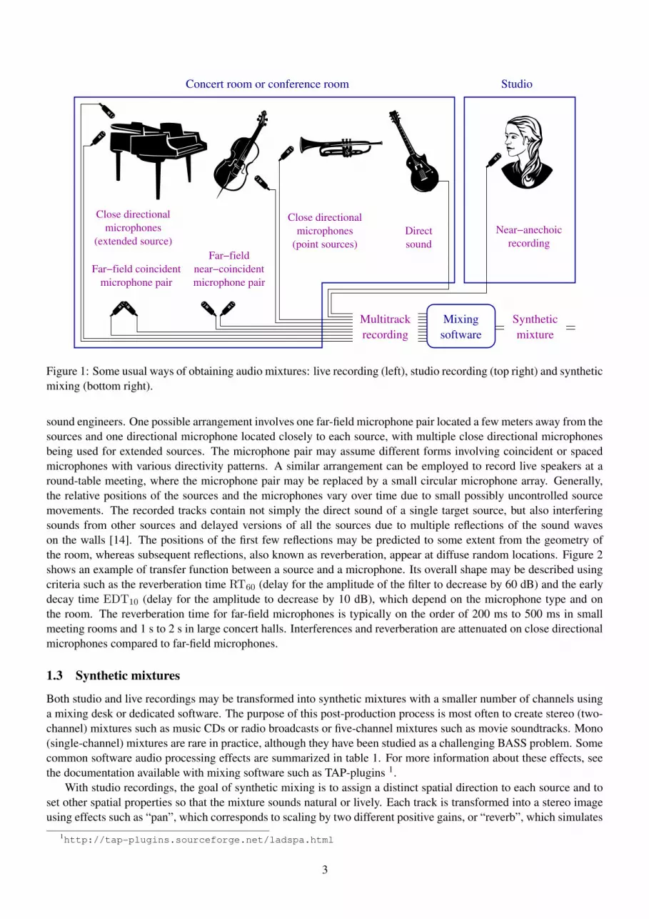
Audio mixtures can be broadly classified into two types: live recordings or synthetic mixtures. The procedure bywhich mixture signals are acquired is depicted in figure 1. Synthetic mixtures are often derived from studio recordings,that is unmixed signals where each source is recorded separately. Since synthetic mixing effects differ from naturalmixing effects obtained by live recording, the two types of mixture signals have noticeably different spatial propertieswhich argue for the use of different processing methods.

A common way of recording multiple sources is to record each one successively in a studio [13]. Point sourcessuch a speakers or small musical instruments, which have a limited spatial extent, are usually recorded using a singleclose microphone. Extended sources such as piano or drums, which can produce distinct sounds in different regions ofspace at the same time, are better recorded using several microphones. This technique is generally employed for popmusic recordings, where the players ensure synchronization by listening on headphones to a mixture of the previouslyrecorded instruments. Similarly, movie dialogues are sometimes dubbed by recording each speaker separately withsynchronization provided by the images. These studio recordings match closely the actual sound of the sourcessince studio walls are covered with sound dampening materials and marginal reflections of the sound waves on thewalls can be limited by using directional microphones. Electric or electronic instruments such as electric guitars andkeyboards may even be recorded together since only the direct sound of each instrument is captured. The advantage ofstudio recordings is that they allow different special effects to be applied to each source because sources are perfectlyseparated into distinct tracks.

By contrast, live recordings contain mixtures of several sources obtained by recording all the sources simultane-ously with multiple microphones [13]. This technique is preferred for classical music because it is more practical forlarge ensembles and it retains the characteristics of the concert room. Various microphone arrangements are used by

2

��

��

��

�� !! !!

"#$$ $$%% %%

Far−fieldnear−coincidentmicrophone pair

Close directionalmicrophones

(extended source)

Close directionalmicrophones

(point sources)

Concert room or conference room Studio

&'(((())))

soundDirect

Mixingsoftware

Multitrackrecording mixture

Synthetic

Far−field coincidentmicrophone pair

recordingNear−anechoic

Figure 1: Some usual ways of obtaining audio mixtures: live recording (left), studio recording (top right) and syntheticmixing (bottom right).

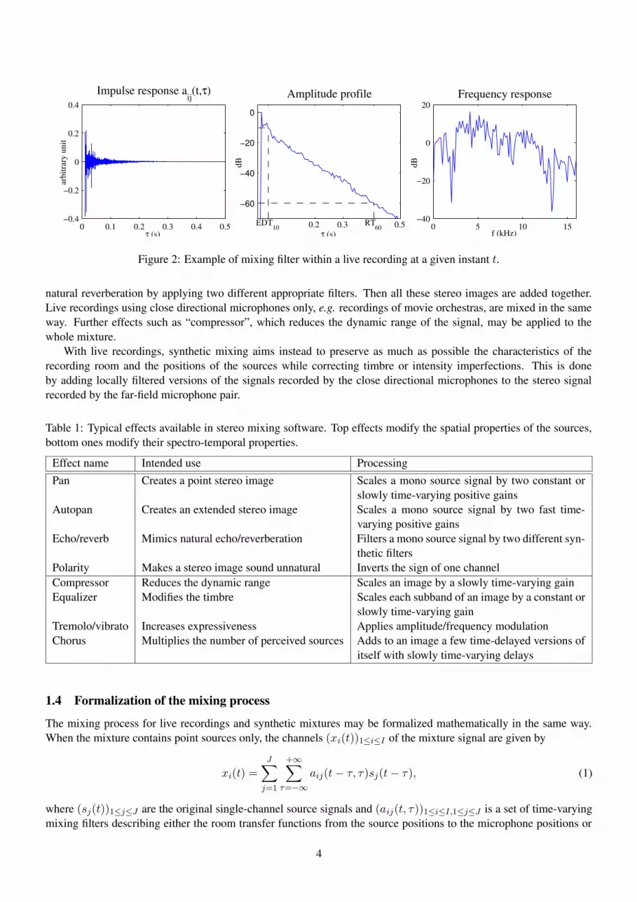
sound engineers. One possible arrangement involves one far-field microphone pair located a few meters away from thesources and one directional microphone located closely to each source, with multiple close directional microphonesbeing used for extended sources. The microphone pair may assume different forms involving coincident or spacedmicrophones with various directivity patterns. A similar arrangement can be employed to record live speakers at around-table meeting, where the microphone pair may be replaced by a small circular microphone array. Generally,the relative positions of the sources and the microphones vary over time due to small possibly uncontrolled sourcemovements. The recorded tracks contain not simply the direct sound of a single target source, but also interferingsounds from other sources and delayed versions of all the sources due to multiple reflections of the sound waveson the walls [14]. The positions of the first few reflections may be predicted to some extent from the geometry ofthe room, whereas subsequent reflections, also known as reverberation, appear at diffuse random locations. Figure 2shows an example of transfer function between a source and a microphone. Its overall shape may be described usingcriteria such as the reverberation time RT60 (delay for the amplitude of the filter to decrease by 60 dB) and the earlydecay time EDT10 (delay for the amplitude to decrease by 10 dB), which depend on the microphone type and onthe room. The reverberation time for far-field microphones is typically on the order of 200 ms to 500 ms in smallmeeting rooms and 1 s to 2 s in large concert halls. Interferences and reverberation are attenuated on close directionalmicrophones compared to far-field microphones.

1.3 Synthetic mixtures

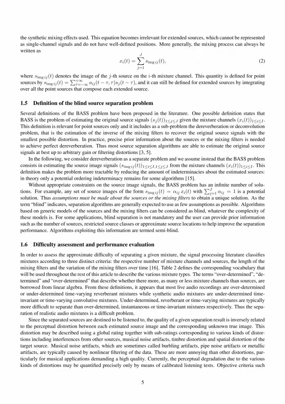
Both studio and live recordings may be transformed into synthetic mixtures with a smaller number of channels usinga mixing desk or dedicated software. The purpose of this post-production process is most often to create stereo (two-channel) mixtures such as music CDs or radio broadcasts or five-channel mixtures such as movie soundtracks. Mono(single-channel) mixtures are rare in practice, although they have been studied as a challenging BASS problem. Somecommon software audio processing effects are summarized in table 1. For more information about these effects, seethe documentation available with mixing software such as TAP-plugins 1.

With studio recordings, the goal of synthetic mixing is to assign a distinct spatial direction to each source and toset other spatial properties so that the mixture sounds natural or lively. Each track is transformed into a stereo imageusing effects such as “pan”, which corresponds to scaling by two different positive gains, or “reverb”, which simulates

1http://tap-plugins.sourceforge.net/ladspa.html

3

0 0.1 0.2 0.3 0.4 0.5−0.4

−0.2

0

0.2

0.4

Impulse response aij(t,τ)

τ (s)

arbi

trar

y un

it

−60

−40

−20

0

Amplitude profile

τ (s)dB

EDT10 0.2 0.3 RT

60 0.5 0 5 10 15−40

−20

0

20Frequency response

f (kHz)

dB

Figure 2: Example of mixing filter within a live recording at a given instant t.

natural reverberation by applying two different appropriate filters. Then all these stereo images are added together.Live recordings using close directional microphones only, e.g. recordings of movie orchestras, are mixed in the sameway. Further effects such as “compressor”, which reduces the dynamic range of the signal, may be applied to thewhole mixture.

With live recordings, synthetic mixing aims instead to preserve as much as possible the characteristics of therecording room and the positions of the sources while correcting timbre or intensity imperfections. This is doneby adding locally filtered versions of the signals recorded by the close directional microphones to the stereo signalrecorded by the far-field microphone pair.

Table 1: Typical effects available in stereo mixing software. Top effects modify the spatial properties of the sources,bottom ones modify their spectro-temporal properties.

Effect name Intended use ProcessingPan Creates a point stereo image Scales a mono source signal by two constant or

slowly time-varying positive gainsAutopan Creates an extended stereo image Scales a mono source signal by two fast time-

varying positive gainsEcho/reverb Mimics natural echo/reverberation Filters a mono source signal by two different syn-

thetic filtersPolarity Makes a stereo image sound unnatural Inverts the sign of one channelCompressor Reduces the dynamic range Scales an image by a slowly time-varying gainEqualizer Modifies the timbre Scales each subband of an image by a constant or

slowly time-varying gainTremolo/vibrato Increases expressiveness Applies amplitude/frequency modulationChorus Multiplies the number of perceived sources Adds to an image a few time-delayed versions of

itself with slowly time-varying delays

1.4 Formalization of the mixing process

The mixing process for live recordings and synthetic mixtures may be formalized mathematically in the same way.When the mixture contains point sources only, the channels (xi(t))1≤i≤I of the mixture signal are given by

xi(t) =J

∑

j=1

+∞∑

τ=−∞

aij(t − τ, τ)sj(t − τ), (1)

where (sj(t))1≤j≤J are the original single-channel source signals and (aij(t, τ))1≤i≤I,1≤j≤J is a set of time-varyingmixing filters describing either the room transfer functions from the source positions to the microphone positions or

4

the synthetic mixing effects used. This equation becomes irrelevant for extended sources, which cannot be representedas single-channel signals and do not have well-defined positions. More generally, the mixing process can always bewritten as

xi(t) =J

∑

j=1

simg ij(t), (2)

where simg ij(t) denotes the image of the j-th source on the i-th mixture channel. This quantity is defined for pointsources by simg ij(t) =

∑+∞τ=−∞ aij(t − τ, τ)sj(t − τ), and it can still be defined for extended sources by integrating

over all the point sources that compose each extended source.

1.5 Definition of the blind source separation problem

Several definitions of the BASS problem have been proposed in the literature. One possible definition states thatBASS is the problem of estimating the original source signals (sj(t))1≤j≤J given the mixture channels (xi(t))1≤i≤I .This definition is relevant for point sources only and it includes as a sub-problem the dereverberation or deconvolutionproblem, that is the estimation of the inverse of the mixing filters to recover the original source signals with thesmallest possible distortion. In practice, precise prior information about the sources or the mixing filters is neededto achieve perfect dereverberation. Thus most source separation algorithms are able to estimate the original sourcesignals at best up to arbitrary gain or filtering distortions [3, 5].

In the following, we consider dereverberation as a separate problem and we assume instead that the BASS problemconsists in estimating the source image signals (simg ij(t))1≤i≤I,1≤j≤J from the mixture channels (xi(t))1≤i≤I . Thisdefinition makes the problem more tractable by reducing the amount of indeterminacies about the estimated sources:in theory only a potential ordering indeterminacy remains for some algorithms [15].

Without appropriate constraints on the source image signals, the BASS problem has an infinite number of solu-tions. For example, any set of source images of the form simg ij(t) = αij xi(t) with

∑Jj=1 αij = 1 is a potential

solution. Thus assumptions must be made about the sources or the mixing filters to obtain a unique solution. As theterm “blind” indicates, separation algorithms are generally expected to use as few assumptions as possible. Algorithmsbased on generic models of the sources and the mixing filters can be considered as blind, whatever the complexity ofthese models is. For some applications, blind separation is not mandatory and the user can provide prior informationsuch as the number of sources, restricted source classes or approximate source locations to help improve the separationperformance. Algorithms exploiting this information are termed semi-blind.

1.6 Difficulty assessment and performance evaluation

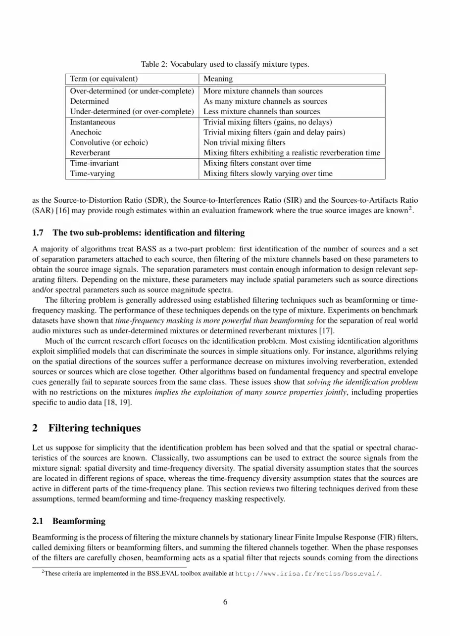
In order to assess the approximate difficulty of separating a given mixture, the signal processing literature classifiesmixtures according to three distinct criteria: the respective number of mixture channels and sources, the length of themixing filters and the variation of the mixing filters over time [16]. Table 2 defines the corresponding vocabulary thatwill be used throughout the rest of this article to describe the various mixture types. The terms “over-determined”, “de-termined” and “over-determined” that describe whether there more, as many or less mixture channels than sources, areborrowed from linear algebra. From these definitions, it appears that most live audio recordings are over-determinedor under-determined time-varying reverberant mixtures while synthetic audio mixtures are under-determined time-invariant or time-varying convolutive mixtures. Under-determined, reverberant or time-varying mixtures are typicallymore difficult to separate than over-determined, instantaneous or time-invariant mixtures respectively. Thus the sepa-ration of realistic audio mixtures is a difficult problem.

Since the separated sources are destined to be listened to, the quality of a given separation result is inversely relatedto the perceptual distortion between each estimated source image and the corresponding unknown true image. Thisdistortion may be described using a global rating together with sub-ratings corresponding to various kinds of distor-tions including interferences from other sources, musical noise artifacts, timbre distortion and spatial distortion of thetarget source. Musical noise artifacts, which are sometimes called burbling artifacts, pipe noise artifacts or metallicartifacts, are typically caused by nonlinear filtering of the data. These are more annoying than other distortions, par-ticularly for musical applications demanding a high quality. Currently, the perceptual degradation due to the variouskinds of distortions may be quantified precisely only by means of calibrated listening tests. Objective criteria such

5

Table 2: Vocabulary used to classify mixture types.

Term (or equivalent) MeaningOver-determined (or under-complete) More mixture channels than sourcesDetermined As many mixture channels as sourcesUnder-determined (or over-complete) Less mixture channels than sourcesInstantaneous Trivial mixing filters (gains, no delays)Anechoic Trivial mixing filters (gain and delay pairs)Convolutive (or echoic) Non trivial mixing filtersReverberant Mixing filters exhibiting a realistic reverberation timeTime-invariant Mixing filters constant over timeTime-varying Mixing filters slowly varying over time

as the Source-to-Distortion Ratio (SDR), the Source-to-Interferences Ratio (SIR) and the Sources-to-Artifacts Ratio(SAR) [16] may provide rough estimates within an evaluation framework where the true source images are known2.

1.7 The two sub-problems: identification and filtering

A majority of algorithms treat BASS as a two-part problem: first identification of the number of sources and a setof separation parameters attached to each source, then filtering of the mixture channels based on these parameters toobtain the source image signals. The separation parameters must contain enough information to design relevant sep-arating filters. Depending on the mixture, these parameters may include spatial parameters such as source directionsand/or spectral parameters such as source magnitude spectra.

The filtering problem is generally addressed using established filtering techniques such as beamforming or time-frequency masking. The performance of these techniques depends on the type of mixture. Experiments on benchmarkdatasets have shown that time-frequency masking is more powerful than beamforming for the separation of real worldaudio mixtures such as under-determined mixtures or determined reverberant mixtures [17].

Much of the current research effort focuses on the identification problem. Most existing identification algorithmsexploit simplified models that can discriminate the sources in simple situations only. For instance, algorithms relyingon the spatial directions of the sources suffer a performance decrease on mixtures involving reverberation, extendedsources or sources which are close together. Other algorithms based on fundamental frequency and spectral envelopecues generally fail to separate sources from the same class. These issues show that solving the identification problemwith no restrictions on the mixtures implies the exploitation of many source properties jointly, including propertiesspecific to audio data [18, 19].

2 Filtering techniques

Let us suppose for simplicity that the identification problem has been solved and that the spatial or spectral charac-teristics of the sources are known. Classically, two assumptions can be used to extract the source signals from themixture signal: spatial diversity and time-frequency diversity. The spatial diversity assumption states that the sourcesare located in different regions of space, whereas the time-frequency diversity assumption states that the sources areactive in different parts of the time-frequency plane. This section reviews two filtering techniques derived from theseassumptions, termed beamforming and time-frequency masking respectively.

2.1 Beamforming

Beamforming is the process of filtering the mixture channels by stationary linear Finite Impulse Response (FIR) filters,called demixing filters or beamforming filters, and summing the filtered channels together. When the phase responsesof the filters are carefully chosen, beamforming acts as a spatial filter that rejects sounds coming from the directions

2These criteria are implemented in the BSS EVAL toolbox available at http://www.irisa.fr/metiss/bss eval/.

6

of interfering sources, which may move depending on frequency. This process is most often expressed in the time-frequency domain. The demixing filters then correspond to a matrix of complex coefficients (wji(f))1≤i≤I,1≤j≤J foreach subband f whose estimation constitutes the inference problem. Let Xi(n, f) be the complex Short-Term FourierTransform (STFT) of the mixture channel xi(t) and Simg ij(n, f) the STFTs of the source image simg ij(t). Theimages (simg ij(t))1≤i≤I of the j-th source on different channels are filtered versions of each other, thus their STFTs(Simg ij(n, f))1≤i≤I are approximately equal to a common STFT Uj(n, f) up to a complex multiplicative coefficientin each subband f . This common STFT is estimated for each source j by

Uj(n, f) =I

∑

i=1

wji(f)Xi(n, f). (3)

Then the STFTs of the source images are derived by computing these multiplicative coefficients with

Simg ij(n, f) = bij(f)Uj(n, f), (4)

where (bij(f))1≤i≤I,1≤j≤J is the pseudo-inverse matrix of (wji(f))1≤i≤I,1≤j≤J . Note that to obtain this result thedemixing coefficients (wji(f))1≤i≤I for each source j need to be specified only up to an arbitrary complex multi-plicative coefficient in each subband f [15]. Finally the source image signals (simg ij(t))1≤i≤I,1≤j≤J are estimatedby inverting their STFTs using the standard overlap-add method.

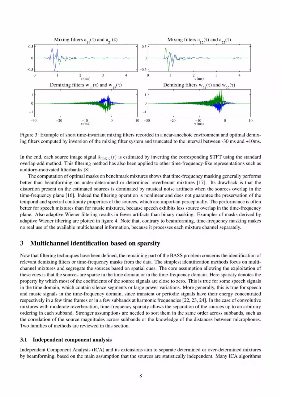
In theory, determined or over-determined mixtures can be perfectly separated using beamforming by constructingthe demixing filter system to be the pseudo-inverse of the mixing filter system. In practice however, the optimaldemixing filters are often much longer than the mixing filters, particularly in the case of determined mixtures, asillustrated in figure 3, and shorter suboptimal filters are used instead. The main advantage of beamforming is thatit does not generate musical noise artifacts since it performs a linear filtering of the data [16]. The computationof optimal demixing filters on benchmark mixtures where the true sources are known3 shows that beamforming canprovide near perfect separation for determined time-invariant mixtures generated by short mixing filters up to the orderof a thousand taps [17]. Conversely beamforming fails on under-determined mixtures and its performance deteriorateson determined reverberant mixtures [17], because the maximal number of directions it can reject is limited by thenumber of mixture channels. In this context, the performance does not increase much by increasing the length of thedemixing filters. Beamforming also fails on determined time-varying mixtures when time-invariant demixing filtersare used since the rejection patterns are too narrow to encompass even small source movements [20]. Robustnesstowards reverberation and source movements improves on over-determined mixtures [21], where the optimal demixingfilters are shorter and can generate wider or more complex rejection patterns.

2.2 Time-frequency masking

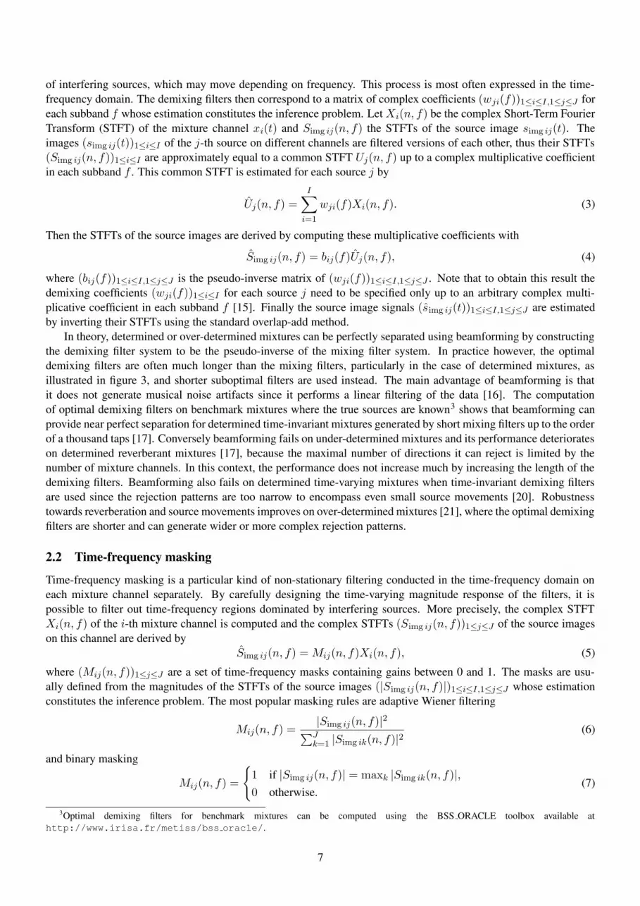
Time-frequency masking is a particular kind of non-stationary filtering conducted in the time-frequency domain oneach mixture channel separately. By carefully designing the time-varying magnitude response of the filters, it ispossible to filter out time-frequency regions dominated by interfering sources. More precisely, the complex STFTXi(n, f) of the i-th mixture channel is computed and the complex STFTs (Simg ij(n, f))1≤j≤J of the source imageson this channel are derived by

Simg ij(n, f) = Mij(n, f)Xi(n, f), (5)

where (Mij(n, f))1≤j≤J are a set of time-frequency masks containing gains between 0 and 1. The masks are usu-ally defined from the magnitudes of the STFTs of the source images (|Simg ij(n, f)|)1≤i≤I,1≤j≤J whose estimationconstitutes the inference problem. The most popular masking rules are adaptive Wiener filtering

Mij(n, f) =|Simg ij(n, f)|2

∑Jk=1 |Simg ik(n, f)|2

(6)

and binary masking

Mij(n, f) =

{

1 if |Simg ij(n, f)| = maxk |Simg ik(n, f)|,

0 otherwise.(7)

3Optimal demixing filters for benchmark mixtures can be computed using the BSS ORACLE toolbox available athttp://www.irisa.fr/metiss/bss oracle/.

7

0 1 2 3 4

−0.5

0

0.5

Mixing filters a11

(τ) and a21

(τ)

τ (ms)0 1 2 3 4

−0.5

0

0.5

Mixing filters a12

(τ) and a22

(τ)

τ (ms)

−30 −20 −10 0 10

−1

0

1

Demixing filters w11

(τ) and w12

(τ)

τ (ms)−30 −20 −10 0 10

−1

0

1

Demixing filters w21

(τ) and w22

(τ)

τ (ms)

Figure 3: Example of short time-invariant mixing filters recorded in a near-anechoic environment and optimal demix-ing filters computed by inversion of the mixing filter system and truncated to the interval between -30 ms and +10ms.

In the end, each source image signal simg ij(t) is estimated by inverting the corresponding STFT using the standardoverlap-add method. This filtering method has also been applied to other time-frequency-like representations such asauditory-motivated filterbanks [8].

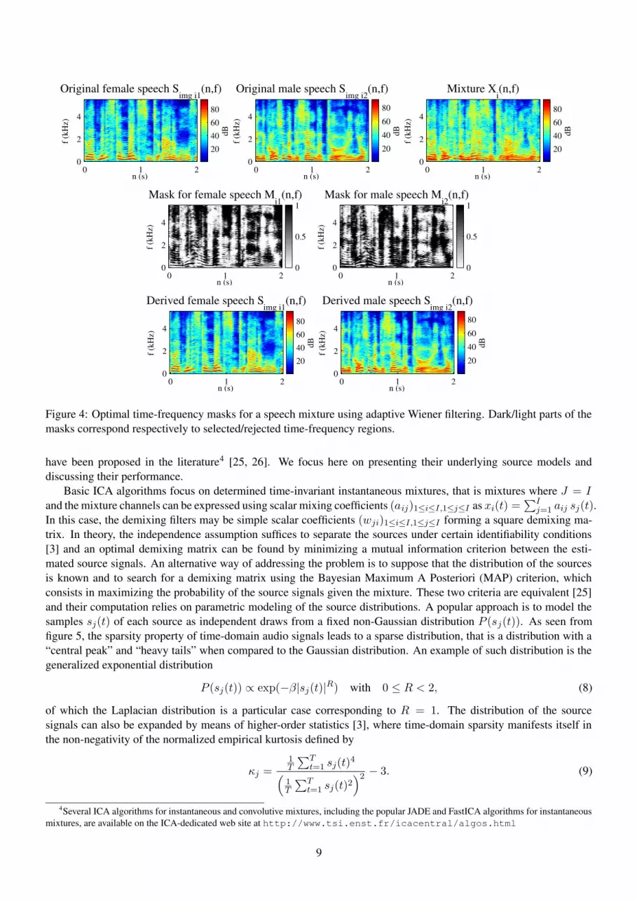
The computation of optimal masks on benchmark mixtures shows that time-frequency masking generally performsbetter than beamforming on under-determined or determined reverberant mixtures [17]. Its drawback is that thedistortion present on the estimated sources is dominated by musical noise artifacts when the sources overlap in thetime-frequency plane [16]. Indeed the filtering operation is nonlinear and does not guarantee the preservation of thetemporal and spectral continuity properties of the sources, which are important perceptually. The performance is oftenbetter for speech mixtures than for music mixtures, because speech exhibits less source overlap in the time-frequencyplane. Also adaptive Wiener filtering results in fewer artifacts than binary masking. Examples of masks derived byadaptive Wiener filtering are plotted in figure 4. Note that, contrary to beamforming, time-frequency masking makesno real use of the available multichannel information, because it processes each mixture channel separately.

3 Multichannel identification based on sparsity

Now that filtering techniques have been defined, the remaining part of the BASS problem concerns the identification ofrelevant demixing filters or time-frequency masks from the data. The simplest identification methods focus on multi-channel mixtures and segregate the sources based on spatial cues. The core assumption allowing the exploitation ofthese cues is that the sources are sparse in the time domain or in the time-frequency domain. Here sparsity denotes theproperty by which most of the coefficients of the source signals are close to zero. This is true for some speech signalsin the time domain, which contain silence segments or large power variations. More generally, this is true for speechand music signals in the time-frequency domain, since transient or periodic signals have their energy concentratedrespectively in a few time frames or in a few subbands at harmonic frequencies [22, 23, 24]. In the case of convolutivemixtures with moderate reverberation, time-frequency sparsity allows the separation of the sources up to an arbitraryordering in each subband. Stronger assumptions are needed to sort them in the same order across subbands, such asthe correlation of the source magnitudes across subbands or the knowledge of the distances between microphones.Two families of methods are reviewed in this section.

3.1 Independent component analysis

Independent Component Analysis (ICA) and its extensions aim to separate determined or over-determined mixturesby beamforming, based on the main assumption that the sources are statistically independent. Many ICA algorithms

8

Original female speech Simg i1

(n,f)

n (s)

f (kH

z)

0 1 20

2

4

dB

20

40

60

80

Original male speech Simg i2

(n,f)

n (s)

f (kH

z)

0 1 20

2

4

dB

20

40

60

80

Mixture Xi(n,f)

n (s)

f (kH

z)

0 1 20

2

4

dB

20

40

60

80

Mask for female speech Mi1

(n,f)

n (s)

f (kH

z)

0 1 20

2

4

0

0.5

1Mask for male speech M

i2(n,f)

n (s)

f (kH

z)

0 1 20

2

4

0

0.5

1

Derived female speech Simg i1

(n,f)

n (s)

f (kH

z)

0 1 20

2

4

dB

20

40

60

80

Derived male speech Simg i2

(n,f)

n (s)

f (kH

z)

0 1 20

2

4

dB

20

40

60

80

Figure 4: Optimal time-frequency masks for a speech mixture using adaptive Wiener filtering. Dark/light parts of themasks correspond respectively to selected/rejected time-frequency regions.

have been proposed in the literature4 [25, 26]. We focus here on presenting their underlying source models anddiscussing their performance.

Basic ICA algorithms focus on determined time-invariant instantaneous mixtures, that is mixtures where J = Iand the mixture channels can be expressed using scalar mixing coefficients (aij)1≤i≤I,1≤j≤I as xi(t) =

∑Ij=1 aij sj(t).

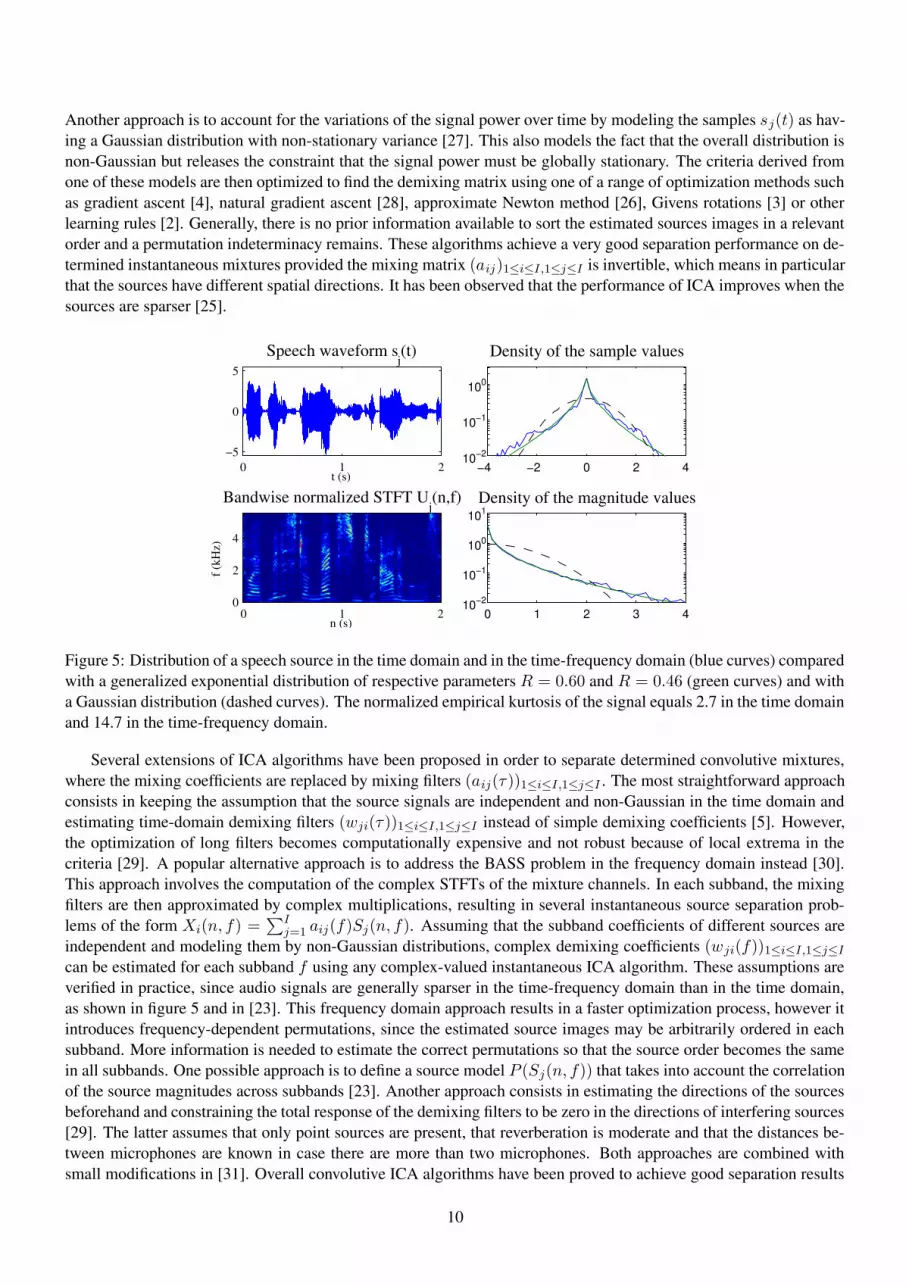
In this case, the demixing filters may be simple scalar coefficients (wji)1≤i≤I,1≤j≤I forming a square demixing ma-trix. In theory, the independence assumption suffices to separate the sources under certain identifiability conditions[3] and an optimal demixing matrix can be found by minimizing a mutual information criterion between the esti-mated source signals. An alternative way of addressing the problem is to suppose that the distribution of the sourcesis known and to search for a demixing matrix using the Bayesian Maximum A Posteriori (MAP) criterion, whichconsists in maximizing the probability of the source signals given the mixture. These two criteria are equivalent [25]and their computation relies on parametric modeling of the source distributions. A popular approach is to model thesamples sj(t) of each source as independent draws from a fixed non-Gaussian distribution P (sj(t)). As seen fromfigure 5, the sparsity property of time-domain audio signals leads to a sparse distribution, that is a distribution with a“central peak” and “heavy tails” when compared to the Gaussian distribution. An example of such distribution is thegeneralized exponential distribution

P (sj(t)) ∝ exp(−β|sj(t)|R) with 0 ≤ R < 2, (8)

of which the Laplacian distribution is a particular case corresponding to R = 1. The distribution of the sourcesignals can also be expanded by means of higher-order statistics [3], where time-domain sparsity manifests itself inthe non-negativity of the normalized empirical kurtosis defined by

κj =1T

∑Tt=1 sj(t)

4

(

1T

∑Tt=1 sj(t)2

)2 − 3. (9)

4Several ICA algorithms for instantaneous and convolutive mixtures, including the popular JADE and FastICA algorithms for instantaneousmixtures, are available on the ICA-dedicated web site at http://www.tsi.enst.fr/icacentral/algos.html

9

Another approach is to account for the variations of the signal power over time by modeling the samples sj(t) as hav-ing a Gaussian distribution with non-stationary variance [27]. This also models the fact that the overall distribution isnon-Gaussian but releases the constraint that the signal power must be globally stationary. The criteria derived fromone of these models are then optimized to find the demixing matrix using one of a range of optimization methods suchas gradient ascent [4], natural gradient ascent [28], approximate Newton method [26], Givens rotations [3] or otherlearning rules [2]. Generally, there is no prior information available to sort the estimated sources images in a relevantorder and a permutation indeterminacy remains. These algorithms achieve a very good separation performance on de-termined instantaneous mixtures provided the mixing matrix (aij)1≤i≤I,1≤j≤I is invertible, which means in particularthat the sources have different spatial directions. It has been observed that the performance of ICA improves when thesources are sparser [25].

0 1 2−5

0

5

Speech waveform sj(t)

t (s)−4 −2 0 2 4

Density of the sample values

10−2

10−1

100

Bandwise normalized STFT Uj(n,f)

n (s)

f (kH

z)

0 1 20

2

4

0 1 2 3 4

Density of the magnitude values

10−2

10−1

100

101

Figure 5: Distribution of a speech source in the time domain and in the time-frequency domain (blue curves) comparedwith a generalized exponential distribution of respective parameters R = 0.60 and R = 0.46 (green curves) and witha Gaussian distribution (dashed curves). The normalized empirical kurtosis of the signal equals 2.7 in the time domainand 14.7 in the time-frequency domain.

Several extensions of ICA algorithms have been proposed in order to separate determined convolutive mixtures,where the mixing coefficients are replaced by mixing filters (aij(τ))1≤i≤I,1≤j≤I . The most straightforward approachconsists in keeping the assumption that the source signals are independent and non-Gaussian in the time domain andestimating time-domain demixing filters (wji(τ))1≤i≤I,1≤j≤I instead of simple demixing coefficients [5]. However,the optimization of long filters becomes computationally expensive and not robust because of local extrema in thecriteria [29]. A popular alternative approach is to address the BASS problem in the frequency domain instead [30].This approach involves the computation of the complex STFTs of the mixture channels. In each subband, the mixingfilters are then approximated by complex multiplications, resulting in several instantaneous source separation prob-lems of the form Xi(n, f) =

∑Ij=1 aij(f)Sj(n, f). Assuming that the subband coefficients of different sources are

independent and modeling them by non-Gaussian distributions, complex demixing coefficients (wji(f))1≤i≤I,1≤j≤I

can be estimated for each subband f using any complex-valued instantaneous ICA algorithm. These assumptions areverified in practice, since audio signals are generally sparser in the time-frequency domain than in the time domain,as shown in figure 5 and in [23]. This frequency domain approach results in a faster optimization process, however itintroduces frequency-dependent permutations, since the estimated source images may be arbitrarily ordered in eachsubband. More information is needed to estimate the correct permutations so that the source order becomes the samein all subbands. One possible approach is to define a source model P (Sj(n, f)) that takes into account the correlationof the source magnitudes across subbands [23]. Another approach consists in estimating the directions of the sourcesbeforehand and constraining the total response of the demixing filters to be zero in the directions of interfering sources[29]. The latter assumes that only point sources are present, that reverberation is moderate and that the distances be-tween microphones are known in case there are more than two microphones. Both approaches are combined withsmall modifications in [31]. Overall convolutive ICA algorithms have been proved to achieve good separation results

10

using demixing filters of a few thousand taps on synthetic time-invariant convolutive mixtures generated with mixingfilters on the order of a thousand taps or live recordings of non-moving sources with moderate reverberation. How-ever their performance decreases fast on realistic mixtures involving more reverberation or small source movements,because of the limitations of beamforming [17, 20].

Convolutive ICA algorithms have also been extended to over-determined convolutive mixtures by applying a sub-space method in each subband to reduce the number of channels I to the number of sources J prior to the applicationof ICA [29]. The resulting performance on over-determined reverberant mixtures is better than with determinedmixtures and increases as a function of the number of mixture channels divided by the number of sources.

3.2 DUET-like methods

In the case of under-determined mixtures, the independence assumption used by ICA becomes insufficient. Moreinformation is needed to estimate the sources and sparsity is often exploited to this end. For instance, instantaneousspeech mixtures can be separated to some extent by modeling the source signals with independent sparse distributionsand jointly optimizing the source signals and the mixing gains with a MAP criterion [32]. This algorithm achievesbetter separation when applied to STFT coefficients [22]. However it is not easily extended to convolutive mixtures.

The Degenerate Unmixing Estimation Technique (DUET) [33] uses a different approach based on the assumptionthat only one source is present in any given time-frequency point. This so-called W-disjoint orthogonality assumptionis expressed mathematically using the STFTs of the source signals as

Sj(n, f)Sj′(n, f) = 0 ∀j 6= j ′, ∀n, f. (10)

Under this assumption, it is possible to determine which source is present in each point from the spatial locationinformation contained in the STFT coefficients of the mixture channels. In the case of stereo mixtures, this informationis given by the Inter-channel Intensity Difference

IID(n, f) = 20 log10

X2(n, f)

X1(n, f)(11)

and the Inter-channel Phase Difference

IPD(n, f) = ∠

(

X2(n, f)

X1(n, f)

)

mod 2π, (12)

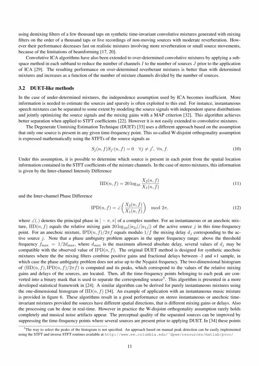
where ∠(.) denotes the principal phase in ] − π, π] of a complex number. For an instantaneous or an anechoic mix-ture, IID(n, f) equals the relative mixing gain 20 log10(|a2j |/|a1j |) of the active source j in this time-frequencypoint. For an anechoic mixture, IPD(n, f)/2πf equals modulo 1/f the mixing delay dj corresponding to the ac-tive source j. Note that a phase ambiguity problem appears in the upper frequency range: above the thresholdfrequency fmax = 1/2dmax, where dmax is the maximum allowed absolute delay, several values of dj may becompatible with the observed value of IPD(n, f). The original DUET method is designed for synthetic anechoicmixtures where the the mixing filters combine positive gains and fractional delays between -1 and +1 sample, inwhich case the phase ambiguity problem does not arise up to the Nyquist frequency. The two-dimensional histogramof (IID(n, f), IPD(n, f)/2πf) is computed and its peaks, which correspond to the values of the relative mixinggains and delays of the sources, are located. Then, all the time-frequency points belonging to each peak are con-verted into a binary mask that is used to separate the corresponding source5. This algorithm is presented in a moredeveloped statistical framework in [24]. A similar algorithm can be derived for purely instantaneous mixtures usingthe one-dimensional histogram of IID(n, f) [34]. An example of application with an instantaneous music mixtureis provided in figure 6. These algorithms result in a good performance on stereo instantaneous or anechoic time-invariant mixtures provided the sources have different spatial directions, that is different mixing gains or delays. Alsothe processing can be done in real-time. However in practice the W-disjoint orthogonality assumption rarely holdscompletely and musical noise artifacts appear. The perceptual quality of the separated sources can be improved bysuppressing the time-frequency points where several sources are present prior to applying DUET. In [34] these points

5The way to select the peaks of the histogram is not specified. An approach based on manual peak detection can be easily implementedusing the STFT and inverse STFT routines available at http://www.ee.columbia.edu/˜dpwe/resources/matlab/pvoc/

11

are located based on the value of the inter-channel coherence, which is the absolute value of the correlation betweenthe coefficients of X1(n, f) and X2(n, f) computed on a small number of successive frames. This quantity is equalto one when a single source is present and it is generally smaller when several sources overlap.

Left mixture channel X11

(n,f)

n (s)

f (kH

z)

0 2 40

5

10

dB

20

40

60

80

IID(n,f)

n (s)f (

kHz)

0 2 40

5

10

dB

−5

0

5

−8 −4 0 4 80

0.5

1

Histogram of IID

Estimated bass drum Simg 11

(n,f)

n (s)

f (kH

z)

0 2 40

5

10

dB

20

40

60

80

Estimated vocals Simg 12

(n,f)

n (s)

f (kH

z)

0 2 40

5

10

dB

20

40

60

80

Estimated bass guitar Simg 13

(n,f)

n (s)

f (kH

z)

0 2 40

5

10

dB

20

40

60

80

Figure 6: Separation of a three-source instantaneous stereo mixture using IID cues and binary masking (sourcescorrespond to IID values of -4, 0 and 4 dB respectively).

The main limitation of DUET is that it cannot deal with realistic convolutive mixtures where the absolute mixingdelay is larger than one sample. In [35], a solution to this problem is provided in the case of stereo convolutivemixtures recorded with a particular microphone pair termed binaural pair, where IID and IPD values are dependenton each other and can be roughly expressed as a function of source direction. The observed direction is estimatedin each time-frequency point based on the IPD value, where IID is exploited in the upper frequency range to solvethe phase ambiguity problem. Then the histogram of directions is computed and the sources are separated by binarymasking as previously. This algorithm is thought to mimic the processing of spatial cues by the auditory system [35].A similar algorithm based on learning the exact average mapping from IID and IPD to source direction is devisedin [36]. The same idea could be exploited for other types of microphone pairs. These DUET-like methods providea good performance on live recordings of non-moving point sources with moderate reverberation. However theirperformance generally decreases in reverberant environments because reverberation effectively adds in interferingsources at random locations. In this situation, interferences are better removed than with ICA, even for determinedmixtures [19].

4 Single-channel identification based on advanced models

As an alternative to multichannel BASS methods based on spatial cues, other authors have studied the separation ofsingle-channel mixtures. In this framework, spatial cues cannot be exploited. Moreover source models relying ontime-frequency sparsity only become insufficient. For example, the W-disjoint orthogonality assumption amounts toassuming that a single source is active in each time-frequency point, but it does not provide enough information todecide which one. More advanced signal models representing the dependencies between the values of the sourcesin various time-frequency points are needed. A first solution is to model the short term waveform of each source.However, this turns out to be difficult, since waveforms are not translation-invariant and vary from recording torecording depending on the phase response of the mixing filters. A popular solution is therefore to model the short-term magnitude spectrum of each source, which has better invariance properties. Note that the modeling of the spectralenvelope alone, which is often used for single-source speech recognition [10], does not provide sufficient informationfor single-channel source separation. Indeed it is necessary to model the harmonicity of the sinusoidal partials ofperiodic sources to separate a mixture of several periodic sources with different fundamental frequencies but with thesame spectral envelope. In addition to the property of correlation of the source magnitudes across subbands, which

12

is used by some convolutive ICA algorithms, advanced models can represent the underlying discrete structures of thesources such as notes and phonemes, along with their fundamental frequency, spectral envelope or temporal continuitycharacteristics. This section reviews three popular models sorted in order of increasing complexity. For simplicity,we drop indices i in the following and we denote by x(t) the signal corresponding to the only mixture channel andby (simg j(t))1≤j≤J the source image signals on this channel, so that x(t) =

∑Jj=1 simg j(t). Similarly, we denote by

X(n, f) and (Simg j(n, f))1≤j≤J the STFTs of the mixture and the source images.

4.1 Factorial hidden Markov models

The simplest signal model used for single-channel BASS is the factorial hidden Markov model (factorial HMM). Letus suppose that the short-term log-power spectrum of the j-th source image is modelled by a HMM with Gaussianobservation densities with shared diagonal covariance. In other words,

log |Simg j(n, f)|2 = Ψhj(n)(f) + εj(n, f), (13)

where hj(n) is a hidden state belonging to a finite space Hj called the state space, Ψhj(n)(f) is a model spectrumdepending on hj(n) and εj(n, f) follows a centered Gaussian distribution whose variance depends on f . Each stategenerally models a particular phoneme at a given fundamental frequency or a particular chord. The sequence of hiddenstates (hj(n))1≤n≤N follows a first order Markov prior defined by the distributions P (hj(1)) and P (hj(n+1)|hj(n)),which model the average duration of each state and the probability of moving from one state to another. A mixtureof several sources may be represented by combining the HMMs representing each source into a single HMM whosehidden states are J-uples of the form h(n) = (h1(n), . . . , hJ(n)). The mixture state space is then the Cartesianproduct H1 × · · · × HJ of the source state spaces. When the sources are assumed to be independent, the priorprobability of the mixture state series factorizes as the product of the prior probabilities of the source state series

P ((h(n))1≤n≤N ) =J

∏

j=1

P (hj(1))N∏

n=2

P (hj(n + 1)|hj(n)), (14)

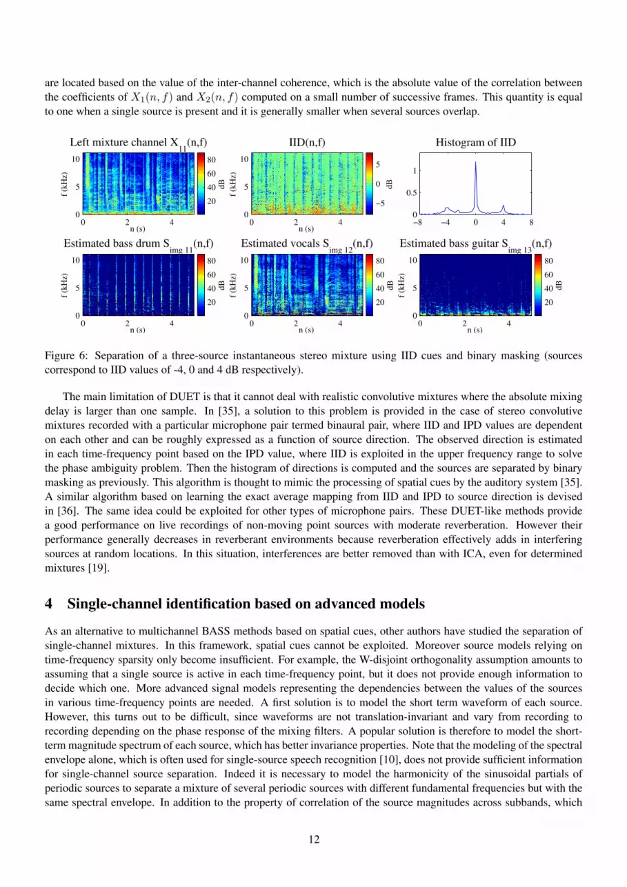
hence the name factorial HMM. The graphical representation of this model is shown in figure 7. Moreover, underthis independence assumption, the power spectrum of the mixture is equal on average to the sum of the source powerspectra and the probability distribution of the short-term log-power spectrum corresponding to each mixture statecan be approximated as a Gaussian density whose mean and covariance are non-trivial functions of the means andcovariances of the underlying source states [37]. In the particular case where all the source observation densities sharethe same diagonal covariance, a simpler approximation is given by the log-max equation [38]

log |X(n, f)|2 ' maxj=1,...,J

Ψhj(n)(f) + ε(n, f), (15)

where ε(n, f) follows a centered Gaussian distribution of the same covariance.

h1(n − 1) h1(n) h1(n + 1) State series for source 1

|X(n − 1, f)|2 |X(n, f)|2 |X(n + 1, f)|2 Observed mixture power spectrum

h2(n − 1) h2(n) h2(n + 1) State series for source 2

Figure 7: Graphical representation of a two-source factorial HMM. Arrows represent conditional dependencies be-tween the variables.

The use of factorial HMMs for single-channel speech separation follows three steps introduced in [38]. Firstly,an individual HMM is trained for each speech source beforehand on solo (single-source) training examples using the

13

EM algorithm. Secondly, the MAP mixture state path (h(n))1≤n≤N is inferred using the Viterbi algorithm alongwith beam search heuristics to avoid computing the posterior probability of improbable paths. These heuristics arenecessary as the size of the mixture state space grows exponentially with the number of sources and an exact estimationis usually intractable. Thirdly, the log-power spectrum of each source image is derived from the source state pathsby log |Simg j(n, f)|2 = Ψ

hj(n)(f) and the corresponding source signals are computed using binary time-frequency

masking6. This algorithm achieves a good separation performance on a mixture of male and female speech.The application of factorial HMMs to the separation of music mixtures raises some difficult issues that are not

encountered with speech mixtures. Most often, the optimal state space underlying music sources is much larger thanfor speech sources because of their wider fundamental frequency and dynamic range as well as their ability to producechords, including chords created by the reverberation of the previous notes in the case of a monophonic instrument.Consequently, HMMs using a small number of states provide a bad separation performance because they model thesources too coarsely. However HMMs using many states provide a bad performance too. Indeed a larger number ofheuristics are needed to maintain the tractability of the inference step and overlearning issues appear: the amount ofdata available to train the parameters of each state becomes so small that the models do not generalize well to dataoutside the training set. In [39], a solution to this problem is provided in the case of mixtures of singing voice andaccompaniment music by segmenting the mixture manually. The HMM representing accompaniment music is trainedon the segments of the mixture containing accompaniment music only, while the HMM representing the singing voiceis first trained on a general corpus of singing voice and then adapted to the mixture using the segments containingboth singing voice and accompaniment music. The resulting separation results are very good given the difficulty ofthe problem, particularly for mixtures with repetitive accompaniment music [39].

4.2 Spectral decomposition

Another way to represent audio sources is to decompose the power spectrum of each source as a weighted sum ofnormalized spectra plus a residual error. For example, the observed spectrum of a note may be represented as aweighted superposition of typical spectra with different spectral envelopes, but with the same fundamental frequencyif periodic, and note spectra may further sum up to yield chord spectra. Again the power spectrum of the single-channel mixture is assumed to be equal to the sum of the source power spectra. This gives

|X(n, f)|2 =

J∑

j=1

Kj∑

k=1

ejk(n)Φjk(f) + ε(n, f), (16)

where (Φjk(f))1≤k≤Kjand (ejk(n))1≤k≤Kj

are respectively the basis spectra and the time-varying weights for eachsource and ε(n, f) is the residual. Generally, weight series from the same source do show some statistical dependen-cies. For example, notes composing a chord are activated at the same time. But weights from different sources areassumed to be independent. This representation is particularly efficient for music sources, because it allows a hugereduction of the model size: only a few basis spectra per note are needed to represent accurately a given source insteadof several model spectra per chord in the case of HMM.

Spectral decomposition has been applied to the separation of music mixtures using a three step data-driven proce-dure. The first step is to derive the MAP basis spectra from the mixture using one of a range of statistical assumptions.An early algorithm [40] represents each series of weights by a sparse distribution and the residual by a Gaussiandistribution. The problem becomes equivalent to over-determined instantaneous ICA and is solved by computing andsubtracting the residual with a subspace technique and applying a standard determined instantaneous ICA algorithm(see Independent component analysis section above). The meaningfulness of the results can be improved by addingthe constraint that the the spectra and the weights are non-negative, which results in a non-negative ICA algorithm[41]. Recently, some authors have pointed out that this non-negativity constraint alone suffices to solve the problem insome situations using a Poisson model for the residual and a Nonnegative Matrix Factorization (NMF) algorithm [42].Also it has been argued that the residual is better modelled as a multiplicative noise which gives more importanceto low-power time-frequency zones [43]. Once the model parameters have been estimated using one of the methods

6These steps can be implemented using the HMM toolbox at http://www.cs.ubc.ca/˜murphyk/Software/HMM/hmm.htmlalong with the above mentioned STFT and inverse STFT routines.

14

above, the second step is to cluster the basis spectra into disjoint sets corresponding to the different sources. Fewalgorithms are able to solve this problem: the Independent Subspace Analysis (ISA) algorithm groups together theweight series that exhibit the highest dependencies [40], while another algorithm employs instrument-specific featuresin the context of drum instruments [44]. Most other algorithms rely on manual clustering. Finally the third step is toderive the power spectrum of each source image by |Simg j(n, f)|2 =

∑Kj

k=1 ejk(n)Φjk(f) and to extract the sourcesignals by time-frequency masking7.

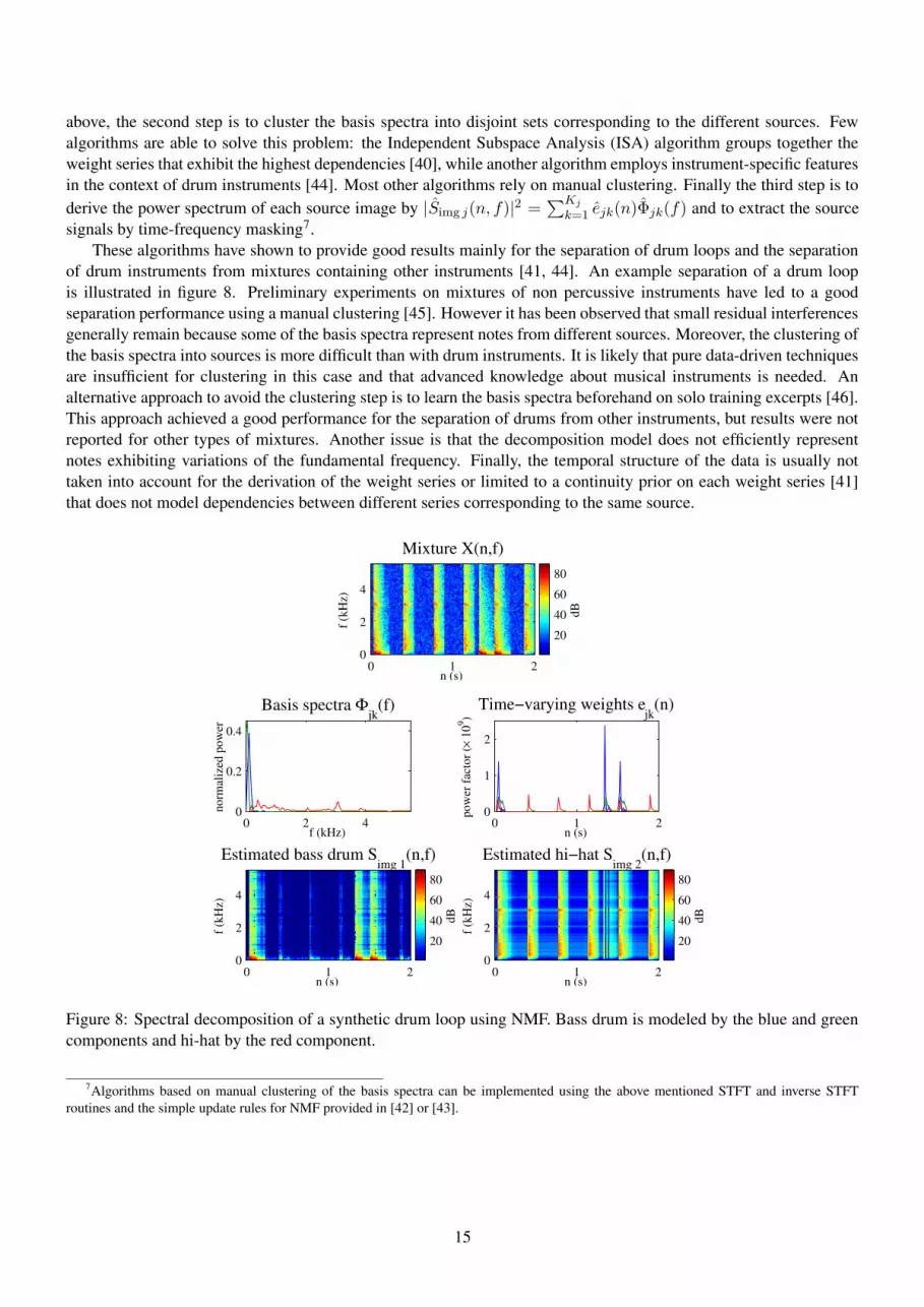
These algorithms have shown to provide good results mainly for the separation of drum loops and the separationof drum instruments from mixtures containing other instruments [41, 44]. An example separation of a drum loopis illustrated in figure 8. Preliminary experiments on mixtures of non percussive instruments have led to a goodseparation performance using a manual clustering [45]. However it has been observed that small residual interferencesgenerally remain because some of the basis spectra represent notes from different sources. Moreover, the clustering ofthe basis spectra into sources is more difficult than with drum instruments. It is likely that pure data-driven techniquesare insufficient for clustering in this case and that advanced knowledge about musical instruments is needed. Analternative approach to avoid the clustering step is to learn the basis spectra beforehand on solo training excerpts [46].This approach achieved a good performance for the separation of drums from other instruments, but results were notreported for other types of mixtures. Another issue is that the decomposition model does not efficiently representnotes exhibiting variations of the fundamental frequency. Finally, the temporal structure of the data is usually nottaken into account for the derivation of the weight series or limited to a continuity prior on each weight series [41]that does not model dependencies between different series corresponding to the same source.

Mixture X(n,f)

n (s)

f (kH

z)

0 1 20

2

4dB

20

40

60

80

0 2 40

0.2

0.4

Basis spectra Φjk

(f)

f (kHz)

norm

aliz

ed p

ower

0 1 20

1

2

Time−varying weights ejk

(n)

n (s)

pow

er fa

ctor

(× 1

09 )

Estimated bass drum Simg 1

(n,f)

n (s)

f (kH

z)

0 1 20

2

4

dB

20

40

60

80

Estimated hi−hat Simg 2

(n,f)

n (s)

f (kH

z)

0 1 20

2

4

dB

20

40

60

80

Figure 8: Spectral decomposition of a synthetic drum loop using NMF. Bass drum is modeled by the blue and greencomponents and hi-hat by the red component.

7Algorithms based on manual clustering of the basis spectra can be implemented using the above mentioned STFT and inverse STFTroutines and the simple update rules for NMF provided in [42] or [43].

15

4.3 Computational auditory scene analysis

Historically, the initial motivation behind spectral decomposition was not to improve the modeling of music sourcesbut to provide a statistical model of hearing organization [40]. The sparsity hypothesis on the time-varying weightsrepresents the belief that the short-time spectrum is reducible to a small number of objects at each instant, each beingmodeled by a stationary spectrum. Audition is known to segregate sources inside a complex scene based on a similarredundancy reduction process [6]. However, auditory objects generally have time-varying spectra, and other cuesare taken into account to group time-frequency zones into objects and stream these objects into sources. Listeningexperiments have led to five grouping/streaming rules called proximity, similarity, continuity, closure and commonfate [6], which corroborate the principles of the Gestalt psychology theory. These rules state for example that a set ofsinusoidal partials constitutes a periodic object only if the partials are harmonic, start and end simultaneously, form asmooth spectral envelope and exhibit similar amplitude and frequency variations. They are sometimes completed bymusic-specific rules defining typical rhythms or fundamental frequency relationships within chords. ComputationalAuditory Scene Analysis (CASA) aims to analyze speech and music mixtures by implementing several of these rulestogether.

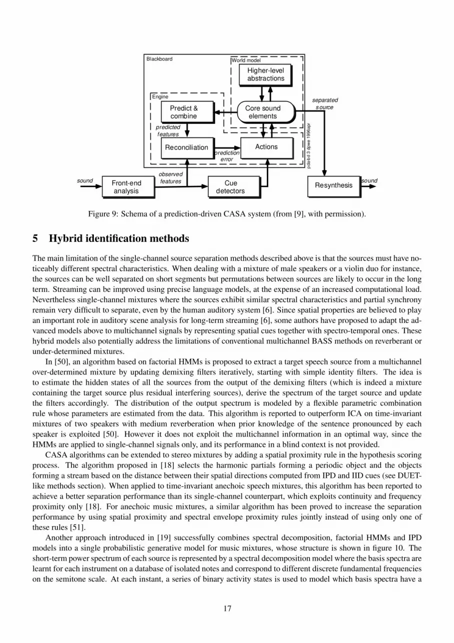
Early CASA algorithms focus on the extraction of objects from single-channel mixtures and contain four succes-sive processing stages [7, 8]. Firstly, the mixture signal is transformed into a front-end representation which is easierto process. Most often, this is done by splitting the signal into several subbands using an auditory-motivated filterbankand computing the autocorrelation function of the absolute value of each subband signal on short time frames, leadingto a three-dimensional representation known as correlogram. For simplicity, this representation is sometimes replacedby a two-dimensional short-term magnitude spectrum [47]. Secondly, a collection of sinusoidal partials is extractedfrom the front-end representation, for example by locating and tracking over time the peaks of the autocorrelationfunction or the magnitude spectrum. Thirdly, these partials are organized iteratively into objects by applying thegrouping rules in a fixed order to the longest remaining partial. Finally, the objects are extracted by binary masking.This data-driven approach lacks some robustness [47, 9]. Indeed, when a given subband contains sinusoidal partialsfrom different sources, the partials corresponding to low power sources may be either not detected at all or transcribedwith erroneous onset times that induce grouping errors due to the rigid evidence integration process. The algorithmin [9] solves this problem by exploiting advanced object models to correct the obscured parameters in a prediction-driven fashion. More precisely, three types of objects called “wefts”, “transients” and “noise clouds” are defined. Forexample, wefts are periodic objects made of perfectly harmonic sinusoidal partials with equal onset and offset timesand constant spectral envelope. Inference is carried out by scanning the time frames in ascending order and testingseveral competing hypotheses (i.e. sets of objects) within a blackboard architecture, as shown in figure 9. The setof hypotheses grows iteratively by prolongating, resuming or creating objects based on harmonicity and onset/offsetcues. Each hypothesis is associated with a score measuring how well the underlying object models fit the observedfront-end representation, and the best scored hypothesis is selected in the end. Note that this prediction-driven ap-proach is close to the Bayesian paradigm where objects are defined by probabilistic priors and their fit to the observeddata is measured by means of a likelihood function. In practice, it is possible to implement similar object models as aBayesian network and to solve the problem by MAP inference [47].

While early CASA algorithms did not consider the streaming of objects into sources, more recent algorithmshave addressed the BASS problem by adding streaming rules in the hypothesis scoring process. One algorithm suitedto mixtures containing one speech source and other non-speech sources searches for the sequence of objects thatresults in the MAP word sequence given a HMM speech model trained on clean speech data [48]. This yields a goodseparation of the speech source when mixed with industrial noise. A similar approach can be devised for mixturescontaining several concurrent speech sources by replacing the single-source HMM with a multi-source factorial HMM.However the problem becomes much more difficult in this case and speaker-specific models may be needed. Otheralgorithms proposed for music mixtures exploit musical knowledge and timbre features learnt on solo excerpts tocluster periodic objects into instruments [47, 49]. These algorithms potentially improve the instrument segregationperformance compared to HMM and spectral decomposition methods since they use advanced timbre features such asonset duration and frequency modulation in addition to the spectral envelope feature. Moreover, they provide a bettermodel for notes with time-varying fundamental frequency.

16

Front-endanalysis

Core soundelements

Predict &combine

Reconciliation

predictedfeatures

Actions

observedfeatures

predictionerror

Higher-levelabstractions

Resynthesis

World modelBlackboard

sound

separatedsource

pda

-bd

3 dp

we

1996

apr

sound

Engine

Cuedetectors

Figure 9: Schema of a prediction-driven CASA system (from [9], with permission).

5 Hybrid identification methods

The main limitation of the single-channel source separation methods described above is that the sources must have no-ticeably different spectral characteristics. When dealing with a mixture of male speakers or a violin duo for instance,the sources can be well separated on short segments but permutations between sources are likely to occur in the longterm. Streaming can be improved using precise language models, at the expense of an increased computational load.Nevertheless single-channel mixtures where the sources exhibit similar spectral characteristics and partial synchronyremain very difficult to separate, even by the human auditory system [6]. Since spatial properties are believed to playan important role in auditory scene analysis for long-term streaming [6], some authors have proposed to adapt the ad-vanced models above to multichannel signals by representing spatial cues together with spectro-temporal ones. Thesehybrid models also potentially address the limitations of conventional multichannel BASS methods on reverberant orunder-determined mixtures.

In [50], an algorithm based on factorial HMMs is proposed to extract a target speech source from a multichannelover-determined mixture by updating demixing filters iteratively, starting with simple identity filters. The idea isto estimate the hidden states of all the sources from the output of the demixing filters (which is indeed a mixturecontaining the target source plus residual interfering sources), derive the spectrum of the target source and updatethe filters accordingly. The distribution of the output spectrum is modeled by a flexible parametric combinationrule whose parameters are estimated from the data. This algorithm is reported to outperform ICA on time-invariantmixtures of two speakers with medium reverberation when prior knowledge of the sentence pronounced by eachspeaker is exploited [50]. However it does not exploit the multichannel information in an optimal way, since theHMMs are applied to single-channel signals only, and its performance in a blind context is not provided.

CASA algorithms can be extended to stereo mixtures by adding a spatial proximity rule in the hypothesis scoringprocess. The algorithm proposed in [18] selects the harmonic partials forming a periodic object and the objectsforming a stream based on the distance between their spatial directions computed from IPD and IID cues (see DUET-like methods section). When applied to time-invariant anechoic speech mixtures, this algorithm has been reported toachieve a better separation performance than its single-channel counterpart, which exploits continuity and frequencyproximity only [18]. For anechoic music mixtures, a similar algorithm has been proved to increase the separationperformance by using spatial proximity and spectral envelope proximity rules jointly instead of using only one ofthese rules [51].

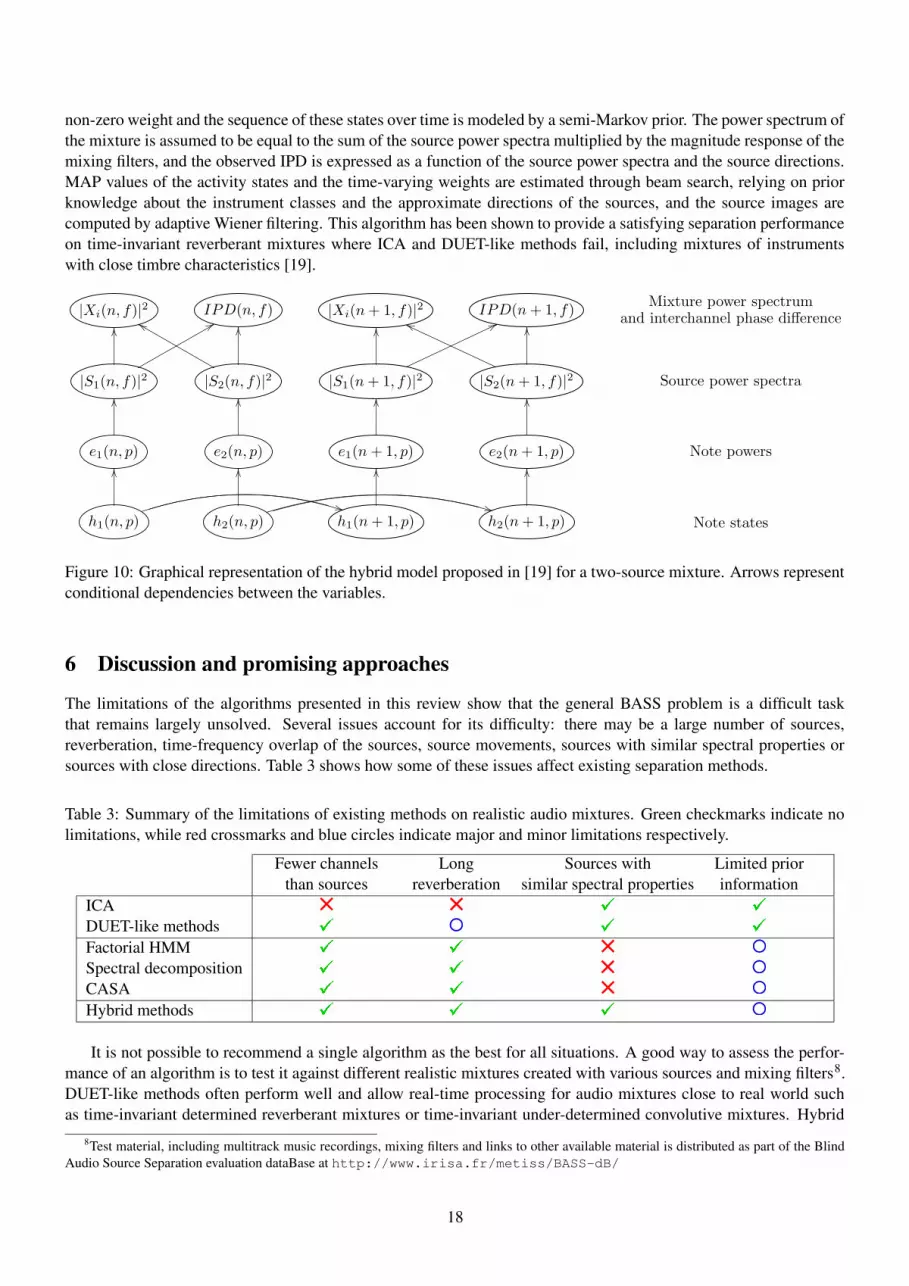
Another approach introduced in [19] successfully combines spectral decomposition, factorial HMMs and IPDmodels into a single probabilistic generative model for music mixtures, whose structure is shown in figure 10. Theshort-term power spectrum of each source is represented by a spectral decomposition model where the basis spectra arelearnt for each instrument on a database of isolated notes and correspond to different discrete fundamental frequencieson the semitone scale. At each instant, a series of binary activity states is used to model which basis spectra have a

17

non-zero weight and the sequence of these states over time is modeled by a semi-Markov prior. The power spectrum ofthe mixture is assumed to be equal to the sum of the source power spectra multiplied by the magnitude response of themixing filters, and the observed IPD is expressed as a function of the source power spectra and the source directions.MAP values of the activity states and the time-varying weights are estimated through beam search, relying on priorknowledge about the instrument classes and the approximate directions of the sources, and the source images arecomputed by adaptive Wiener filtering. This algorithm has been shown to provide a satisfying separation performanceon time-invariant reverberant mixtures where ICA and DUET-like methods fail, including mixtures of instrumentswith close timbre characteristics [19].

|Xi(n, f)|2 IPD(n, f) |Xi(n + 1, f)|2 IPD(n + 1, f)Mixture power spectrum

and interchannel phase difference

|S1(n, f)|2 |S2(n, f)|2 |S1(n + 1, f)|2 |S2(n + 1, f)|2 Source power spectra

e1(n, p) e2(n, p) e1(n + 1, p) e2(n + 1, p) Note powers

h1(n, p) h2(n, p) h1(n + 1, p) h2(n + 1, p) Note states

Figure 10: Graphical representation of the hybrid model proposed in [19] for a two-source mixture. Arrows representconditional dependencies between the variables.

6 Discussion and promising approaches

The limitations of the algorithms presented in this review show that the general BASS problem is a difficult taskthat remains largely unsolved. Several issues account for its difficulty: there may be a large number of sources,reverberation, time-frequency overlap of the sources, source movements, sources with similar spectral properties orsources with close directions. Table 3 shows how some of these issues affect existing separation methods.

Table 3: Summary of the limitations of existing methods on realistic audio mixtures. Green checkmarks indicate nolimitations, while red crossmarks and blue circles indicate major and minor limitations respectively.

Fewer channels Long Sources with Limited priorthan sources reverberation similar spectral properties information

ICADUET-like methodsFactorial HMMSpectral decompositionCASAHybrid methods

It is not possible to recommend a single algorithm as the best for all situations. A good way to assess the perfor-mance of an algorithm is to test it against different realistic mixtures created with various sources and mixing filters8.DUET-like methods often perform well and allow real-time processing for audio mixtures close to real world suchas time-invariant determined reverberant mixtures or time-invariant under-determined convolutive mixtures. Hybrid

8Test material, including multitrack music recordings, mixing filters and links to other available material is distributed as part of the BlindAudio Source Separation evaluation dataBase at http://www.irisa.fr/metiss/BASS-dB/

18

methods exploiting spatial and spectro-temporal cues jointly may perform better, but they are much slower and theymay need more prior information. In the end, the separation quality provided by both types of methods remainsinsufficient for demanding applications such as hearing aids or karaoke.

Recently, two promising approaches have been proposed to overcome these performance limitations. The firstapproach is to investigate new filtering methods. The study of optimal demixing filters and time-frequency masksconducted in [17] has proved that time-frequency masking is a better choice than beamforming for under-determinedmixtures or determined reverberant mixtures. However its performance remains limited by source overlap in the time-frequency plane, partly because each mixture channel is processed separately. Better performance could be achievedby partitioning the time-frequency plane according to the prominent sources and applying different demixing filtersin each zone, thus making full use of the available multichannel information. An advanced source model is neededto perform this partition. The hybrid filtering technique for music mixtures proposed in [52] addresses this problemusing a three-step procedure. First the mixture is separated by the DUET method. Then the time-varying fundamentalfrequency of each source is computed and time-frequency zones containing partials from several sources are detected.Finally each of these zones is separated by adapting complex frequency demixing coefficients so that the amplitudeenvelopes of the separated partials are maximally correlated with the amplitude envelopes of the neighboring partialsthat were well separated in the first step. This technique was shown to improve the separation performance over DUETalone.

The second approach is to build advanced models of the source waveforms, so that the sources can be directlysynthesized from the identified parameters. A popular model is the harmonic sinusoidal model which represents eachsource by a sum of sinusoidal partials with harmonic frequencies and different amplitudes and phases. Overlappingpartials from different sources can be separated using some constraints on the amplitudes. Constraints proposed inthe literature include smoothness of the temporal and spectral envelopes [53] and fixed temporal envelopes learnton isolated notes [54]. The latter leads to good separation results on a mixture of piano and voice, exploiting thescore of the piano part. Sinusoidal models have also been employed by some CASA methods [9, 18]. Becausesinusoidal modeling cannot represent all kinds of sounds, other methods have added complementary models to copewith transient or stationary wideband noise. Several strategies to separate noisy sounds produced by different sourceshave been compared in [55], including an autoregressive model for separating transient from stationary content, abandwise noise power interpolation method for separating overlapping transient noises and a method that uses thecorrelation between the amplitudes of the harmonic partials and the shape of the spectral envelope of the noise. Otherimprovements could include a model for slightly inharmonic partials that are found in many musical instruments suchas piano. Another promising waveform model represents short term frames of the sources as weighted sums of basiswaveforms, in the spirit of spectral decomposition. No constraints are set, so that all kinds of sounds can be modeled.The best waveform basis is learnt directly from the mixture in order to maximize the sparsity of the time-varyingweights under a translational invariance constraint [56]. Preliminary source separation results are not so good, butpotential for improvement exists. In particular, this method could provide a nice model of transient non-noisy sounds.

Other challenging problems remain open. For example, proper modeling of the mixing filters accounting forsource movements could provide major performance improvements on difficult real world mixtures such as musicCDs or speech mixtures recorded in rooms with standard reverberation.

Acknowledgements

Emmanuel Vincent, Maria G. Jafari and Samer A. Abdallah are funded by EPSRC grants GR/S75802/01, GR/S85900/01and GR/S82213/01 respectively. The authors wish to thank Katy Noland and Andrew Nesbit for their useful commentsabout early versions of this article.

References

[1] M. S. Brandstein and D. B. Ward, Eds., Microphone Arrays: Signal Processing Techniques and Applications.Springer Verlag, 2001.

19

[2] J. Herault and C. Jutten, “Space or time adaptive signal processing by neural network models,” in Proc. AmericanInstitute of Physics (AIP) Conf., Snowbird, UT, 1986, pp. 206–211.

[3] P. Comon, “Independent component analysis - a new concept?” Signal Processing, vol. 36, no. 3, pp. 287–314,1994.

[4] A. J. Bell and T. J. Sejnowski, “An information maximization approach to blind separation and blind deconvolu-tion,” Neural Computation, vol. 7, pp. 1129–1159, 1995.

[5] K. Torkkola, “Blind separation of convolved sources based on information maximization,” in Proc. IEEE Work-shop on Neural Networks for Signal Processing (NNSP), 1996, pp. 423–432.

[6] A. S. Bregman, Auditory Scene Analysis. Cambridge, MA: MIT Press, 1990.

[7] D. K. Mellinger, “Event formation and separation in musical sound,” Ph.D. dissertation, CCRMA, StanfordUniversity, 1991.

[8] G. J. Brown and M. P. Cooke, “Computational auditory scene analysis,” Computer Speech and Language, vol. 8,pp. 297–336, 1994.

[9] D. P. W. Ellis, “Prediction-driven computational auditory scene analysis,” Ph.D. dissertation, Dept. of ElectricalEngineering and Computer Science, MIT, 1996.

[10] L. Deng and D. O’Shaughnessy, Speech Processing: A Dynamic and Optimization-Oriented Approach, ser.Signal Processing and Communications. Marcel Dekker, Taylor & Francis, 2003.

[11] D. E. Hall, Musical Acoustics, 3rd Edition. Brooks Cole, 2001.

[12] B. Gygi, G. R. Kidd, and C. S. Watson, “Spectral-temporal factors in the identification of environmental sounds,”Journal of the Acoustical Society of America, vol. 115, no. 3, pp. 1252–1265, 2004.

[13] B. Bartlett and J. Bartlett, Practical Recording Techniques, 4th Edition : the Step-by-step Approach to Profes-sional Recording. Focal Press, 2005.

[14] H. Kuttruff, Room Acoustics, 4th Edition. Spon Press, 2000.

[15] K. Matsuoka and S. Nakashima, “Minimal distortion principle for blind source separation,” in Proc. Int. Conf.on Independent Component Analysis and Blind Source Separation (ICA), 2001, pp. 722–727.

[16] E. Vincent, R. Gribonval, and C. Fevotte, “Performance measurement in blind audio source separation,” IEEETrans. on Speech and Audio Processing, vol. 14, no. 4, 2006, to appear.

[17] E. Vincent and R. Gribonval, “Construction d’estimateurs oracles pour la separation de sources,” in Proc. 20thGRETSI Symposium on Signal and Image Processing, 2005, pp. 1245–1248.

[18] T. Nakatani, “Computational auditory scene analysis based on residue-driven architecture and its applicationto mixed speech recognition,” Ph.D. dissertation, Dept. of Applied Analysis and Complex Dynamical Systems,Kyoto University, 2002.

[19] E. Vincent, “Musical source separation using time-frequency source priors,” IEEE Trans. on Speech and AudioProcessing, vol. 14, no. 1, 2006, to appear.

[20] R. V. Balan, J. P. Rosca, and S. T. Rickard, “Robustness of parametric source demixing in echoic environments,”in Proc. Int. Conf. on Independent Component Analysis and Blind Source Separation (ICA), 2001, pp. 144–148.

[21] A. Westner and V. M. Bove, “Blind separation of real world audio signals using overdetermined mixtures,” inProc. Int. Conf. on Independent Component Analysis and Blind Source Separation (ICA), 1999, pp. 251–256.

20

[22] M. Zibulevsky, B. A. Pearlmutter, P. Bofill, and P. Kisilev, “Blind source separation by sparse decomposition ina signal dictionary,” in Independent Component Analysis : Principles and Practice. Cambridge Press, 2001,pp. 181–208.

[23] M. E. Davies, “Audio source separation,” in Mathematics in Signal Processing V. Oxford University Press,2002.

[24] O. Yilmaz and S. T. Rickard, “Blind separation of speech mixtures via time-frequency masking,” IEEE Trans.on Signal Processing, vol. 52, no. 7, pp. 1830–1847, 2004.

[25] J.-F. Cardoso, “Blind source separation : statistical principles,” Proceedings of the IEEE, vol. 9, no. 10, pp.2009–2025, 1998.

[26] A. Hyvarinen, J. Karhunen, and E. Oja, Independent Component Analysis. John Wiley & Sons, 2001.

[27] D.-T. Pham and J.-F. Cardoso, “Blind separation of instantaneous mixtures of non stationary sources,” IEEETrans. on Signal Processing, vol. 49, no. 9, pp. 1837–1848, 2001.

[28] S.-I. Amari, A. Cichocki, and H. H. Yang, “A new learning algorithm for blind signal separation,” in Advancesin Neural Information Processing Systems (NIPS 8), 1996, pp. 752–763.

[29] L. C. Parra and C. V. Alvino, “Geometric source separation : merging convolutive source separation with geo-metric beamforming,” IEEE Trans. on Speech and Audio Processing, vol. 10, no. 6, pp. 352–362, 2002.

[30] P. Smaragdis, “Blind separation of convolved mixtures in the frequency domain,” Neurocomputing, vol. 22, pp.21–34, 1998.

[31] H. Sawada, R. Mukai, S. Araki, and S. Makino, “A robust and precise method for solving the permutationproblem of frequency-domain blind source separation,” IEEE Trans. on Speech and Audio Processing, vol. 12,no. 5, pp. 530–538, 2004.

[32] T.-W. Lee, M. S. Lewicki, M. A. Girolami, and T. J. Sejnowski, “Blind source separation of more sources thanmixtures using overcomplete representations,” IEEE Signal Processing Letters, vol. 6, no. 4, pp. 87–90, 1999.

[33] A. N. Jourjine, S. T. Rickard, and O. Yilmaz, “Blind separation of disjoint orthogonal signals: Demixing Nsources from 2 mixtures,” in Proc. IEEE Int. Conf. on Acoustics, Speech, and Signal Processing (ICASSP),2000, pp. V–2985–2988.

[34] C. Avendano and J.-M. Jot, “Frequency domain techniques for stereo to multichannel upmix,” in Proc. AES 22ndConference on Vitual, Synthetic and Entertainment Audio, 2002, pp. 121–130.

[35] H. Viste and G. Evangelista, “On the use of spatial cues to improve binaural source separation,” in Proc. Int.Conf. on Digital Audio Effects (DAFx), 2003, pp. 209–213.

[36] N. Roman, D. Wang, and G. J. Brown, “Speech segregation based on sound localization,” Journal of the ASA,vol. 114, no. 4, pp. 2236–2252, 2003.

[37] M. J. F. Gales, “Model-based techniques for noise robust speech recognition,” Ph.D. dissertation, University ofCambridge, 1995.

[38] S. T. Roweis, “One microphone source separation,” in Advances in Neural Information Processing Systems(NIPS 13), 2001, pp. 793–799.

[39] A. Ozerov, P. Philippe, R. Gribonval, and F. Bimbot, “One microphone singing voice separation using source-adapted models,” in Proc. IEEE Workshop on Applications of Signal Processing to Audio and Acoustics (WAS-PAA), 2005, pp. 90–93.

21

[40] M. A. Casey and A. Westner, “Separation of mixed audio sources by independent subspace analysis,” in Proc.Int. Computer Music Conf. (ICMC), 2000, pp. 154–161.

[41] T. Virtanen, “Sound source separation using sparse coding with temporal continuity objective,” in Proc. Int.Computer Music Conf. (ICMC), 2003, pp. 231–234.

[42] P. Smaragdis and J. C. Brown, “Non-negative matrix factorization for polyphonic music transcription,” in Proc.IEEE Workshop on Applications of Signal Processing to Audio and Acoustics (WASPAA), 2003, pp. 177–180.

[43] S. A. Abdallah and M. D. Plumbley, “Polyphonic transcription by non-negative sparse coding of power spectra,”in Proc. Int. Conf. on Music Information Retrieval (ISMIR), 2004, pp. 318–325.

[44] C. Uhle, C. Dittmar, and T. Sporer, “Extraction of drum tracks from polyphonic music using independent sub-space analysis,” in Proc. Int. Conf. on Independent Component Analysis and Blind Source Separation (ICA),2003, pp. 843–848.

[45] B. Wang and M. D. Plumbley, “Musical audio stream separation by non-negative matrix factorization,” in Proc.UK Digital Music Research Network (DMRN) Summer Conf., 2005.

[46] L. Benaroya, L. McDonagh, F. Bimbot, and R. Gribonval, “Non negative sparse representation for Wiener basedsource separation with a single sensor,” in Proc. IEEE Int. Conf. on Acoustics, Speech and Signal Processing(ICASSP), 2004, pp. VI–613–616.

[47] K. Kashino, K. Nakadai, T. Kinoshita, and H. Tanaka, “Application of bayesian probability network to musicscene analysis,” in Working notes of Int. Joint Conf. on Artificial Intelligence (IJCAI) Workshop on Computa-tional Auditory Scene Analysis, 1995, pp. 52–59.

[48] J. P. Barker, M. P. Cooke, and D. P. W. Ellis, “Decoding speech in the presence of other sources,” SpeechCommunication, vol. 45, pp. 5–25, 2005.

[49] T. Kinoshita, S. Sakai, and H. Tanaka, “Musical sound source identification based on frequency componentadaptation,” in Proc. Int. Joint Conf. on Artificial Intelligence (IJCAI) Workshop on Computational AuditoryScene Analysis, 1999, pp. 18–24.

[50] M. J. Reyes-Gomez, B. Raj, and D. P. W. Ellis, “Multi-channel source separation by factorial HMMs,” in Proc.IEEE Int. Conf. on Acoustics, Speech and Signal Processing (ICASSP), 2003, pp. I–664–667.

[51] Y. Sakuraba and H. G. Okuno, “Note recognition of polyphonic music by using timbre similarity and directionproximity,” in Proc. Int. Computer Music Conf. (ICMC), 2003, pp. 167–170.

[52] H. Viste and G. Evangelista, “An extension for source separation techniques avoiding beats,” in Proc. Int. Conf.on Digital Audio Effects (DAFx), 2002, pp. 71–75.

[53] T. Virtanen, “Algorithm for the separation of harmonic sounds with time-frequency smoothness constraint,” inProc. Int. Conf. on Digital Audio Effects (DAFx), 2003, pp. 35–40.

[54] Y. Meron and K. Hirose, “Separation of singing and piano sounds,” in Proc. Int. Conf. on Spoken LanguageProcessing (ICSLP), vol. 3, 1998, pp. 1059–1062.

[55] M. R. Every, “Separating harmonic and inharmonic note content from real mono recordings,” in Proc. UK DigitalMusic Research Network (DMRN) Summer Conf., 2005.

[56] T. Blumensath and M. E. Davies, “Unsupervised learning of sparse and shift-invariant decompositions of poly-phonic music,” in Proc. IEEE Int. Conf. on Acoustics, Speech and Signal Processing (ICASSP), 2004, pp. V–497–500.

22

Date post:	19-Nov-2023
Category:	Documents
Upload:	surrey
View:	2 times
Download:	0 times

Blind Audio Source Separation

Documents